Make a raster plot of a matrix. — matrix_raster

Given a matrix mat, make a raster plot of the matrix whereby in the plot, the pixel at \(x = \)i, \(y = \)j has colour based on the value of mat[i, j] and the \(x\) axis points right and the \(y\) axis points down (see 'Details').

Usage

matrix_raster_plot(
  mat,
  scale_name = "scale",
  limits = NULL,
  ranges = NULL,
  range_names = NULL,
  colours = NULL,
  na_colour = "black",
  clip = FALSE,
  clip_low = FALSE,
  clip_high = FALSE,
  log_trans = FALSE,
  breaks = NULL,
  include_breaks = NULL
)

Arguments

mat

The matrix you wish to plot.

scale_name

A string. The title of the color scale on the right of the plot.

limits

This gives the user the option to set all values outside a certain range to their nearest value within that range (if clip = TRUE) or to NA (if clip = FALSE. For example, to set all values outside the range [1.5, 2.6) to NA, use limits = c(1.5, 2.6), clip = FALSE. The colour range will cover all values within these specified limits.

ranges

A numeric vector. If you want specific ranges of values to have the same color, specify these ranges via an increasing numeric vector. For example, if you want the ranges 0.5-1.2 and 1.2-3, use ranges = c(0.5, 1.2, 3). If ranges is specified as a number (a numeric vector of length 1) n, this is equivalent to setting ranges to be n equal-length intervals within the range of the matrix, i.e. it is equivalent to setting `ranges = seq(min(mat), max(mat), length.out = n

1). At most one of rangesandlimitsshould be set. If ranges is set, the behaviour for values which are not in any of the ranges are set by thecliparguments as in thelimits` argument.

range_names

A character vector. If your colour scale is discrete, here you can set the names which will label each range in the legend.

colours

If you have set ranges, here you may specify which colors you wish to colour each range. It must have the same length as the number of intervals you have specified in ranges. If you have not specified ranges, here you may specify the colours (to be passed to ggplot2::scale_fill_gradientn()) to create the continuous colour band. It is specified as a character vector, with the colors specified either as the values in colors() or as in the value of the rgb() function. Note that this allows the use of grDevices::rainbow() and friends. The default uses viridis::viridis().

na_colour

Which colour should the NA pixels be? Default is black.

clip

If either limits or ranges are set (one should never set both), there may be values that fall outside the specified limits/ranges. If clip = TRUE, values outside these limits/ranges are set to their nearest values within them, but if clip = FALSE, these values are set to NA. Note that setting clip = TRUE is equivalent to setting both clip_low and clip_high to TRUE.

clip_low

Setting this to TRUE (and leaving clip = FALSE, clip_high = FALSE) will set all values falling below the specified limits/ranges to their nearest value within them, but all values falling above those limits/ranges will be set to NA.

clip_high

Setting this to TRUE (and leaving clip = FALSE, clip_low = FALSE) will set all values falling above the specified limits/ranges to their nearest value within them, but all values falling below those limits/ranges will be set to NA.

log_trans

Do you want to log-transform the colour scaling?

breaks

Where do you want tick marks to appear on the legend colour scale?

include_breaks

If you don't want to specify all the breaks, but you want some specific ones to be included on the legend colour scale, specify those specific ones here.

Value

In the graphics console, a raster plot (via ggplot2::geom_raster()) will appear with the matrix values represented as pixel colours, with a named scale bar.

Examples

# \donttest{
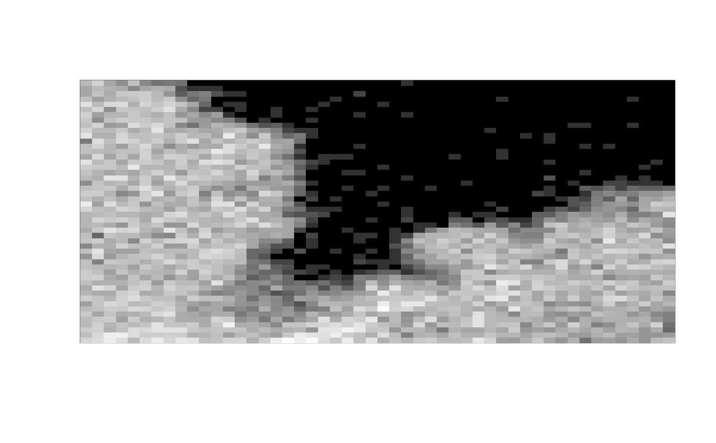
img <- ijtiff::read_tif(system.file("extdata", "50.tif", package = "nandb"))
#> Reading 50.tif: an 8-bit, 50x50 pixel image of unsigned
#> integer type. Reading 1 channel and 50 frames . . .
#> Done.
ijtiff::display(img[, , 1, 1])
#> Using basic display functionality.
#>   * For better display functionality, install the EBImage package.
#>   * To install `EBImage`:
#>     - Install `BiocManager` with `install.packages("BiocManager")`.
#>     - Then run `BiocManager::install("EBImage")`.

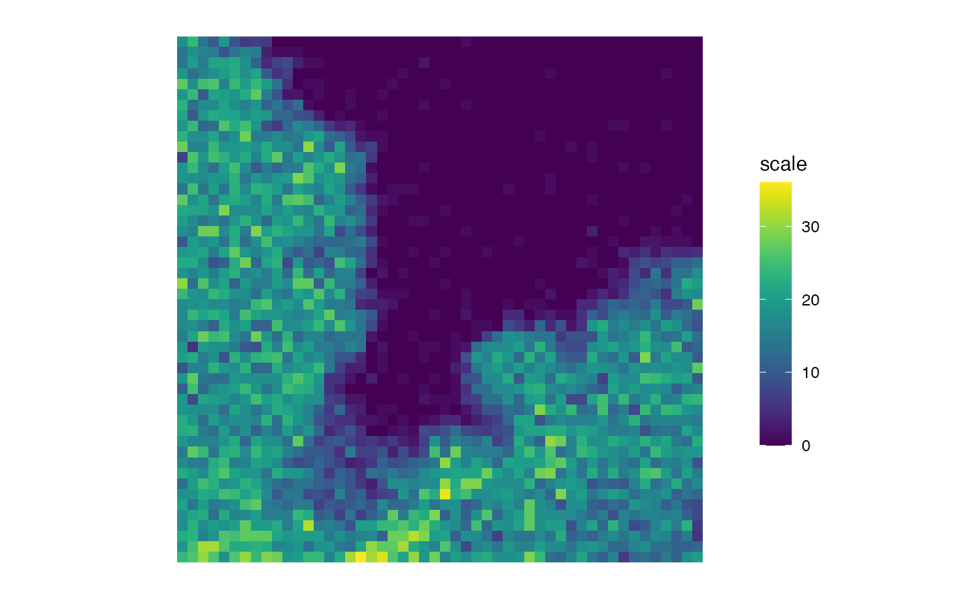
matrix_raster_plot(img[, , 1, 1])

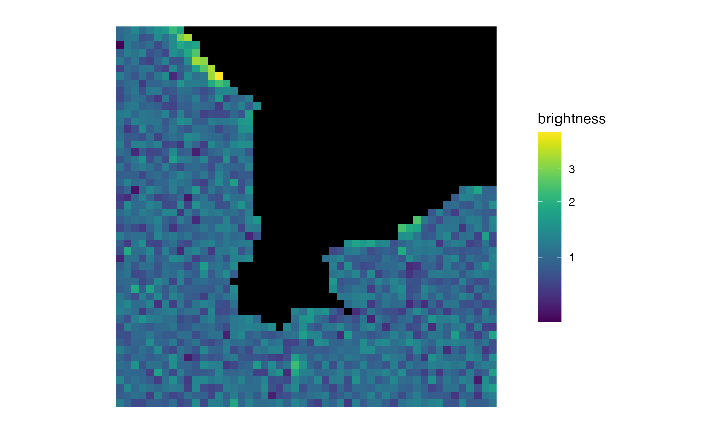
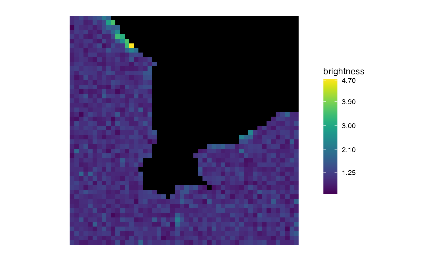
b <- brightness(img, def = "B", detrend = FALSE, thresh = "Huang")
matrix_raster_plot(b, scale_name = "brightness")

matrix_raster_plot(b, scale_name = "brightness", log_trans = TRUE)

matrix_raster_plot(b,
  scale_name = "brightness", log_trans = TRUE,
  include_breaks = 1.35
)

matrix_raster_plot(b,
  scale_name = "brightness", log_trans = TRUE,
  breaks = 1:3
)

matrix_raster_plot(b,
  scale_name = "brightness",
  ranges = seq(0.5, 3, length.out = 6),
  range_names = paste0(1:5, "mer")
)

matrix_raster_plot(b,
  scale_name = "brightness",
  ranges = seq(0.5, 3, length.out = 6),
  range_names = paste0(1:5, "mer"), log_trans = TRUE
)

matrix_raster_plot(b,
  scale_name = "brightness",
  include_breaks = 1.25, range_names = NULL,
  log_trans = FALSE
)

matrix_raster_plot(b,
  scale_name = "brightness",
  include_breaks = 1.25, log_trans = TRUE
)

matrix_raster_plot(b,
  scale_name = "brightness",
  limits = c(1, 1.25), clip = TRUE
)

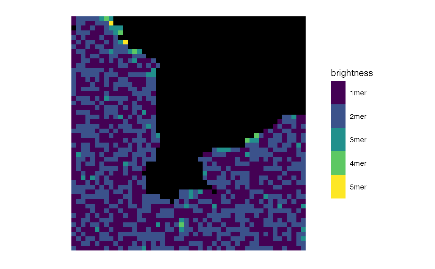
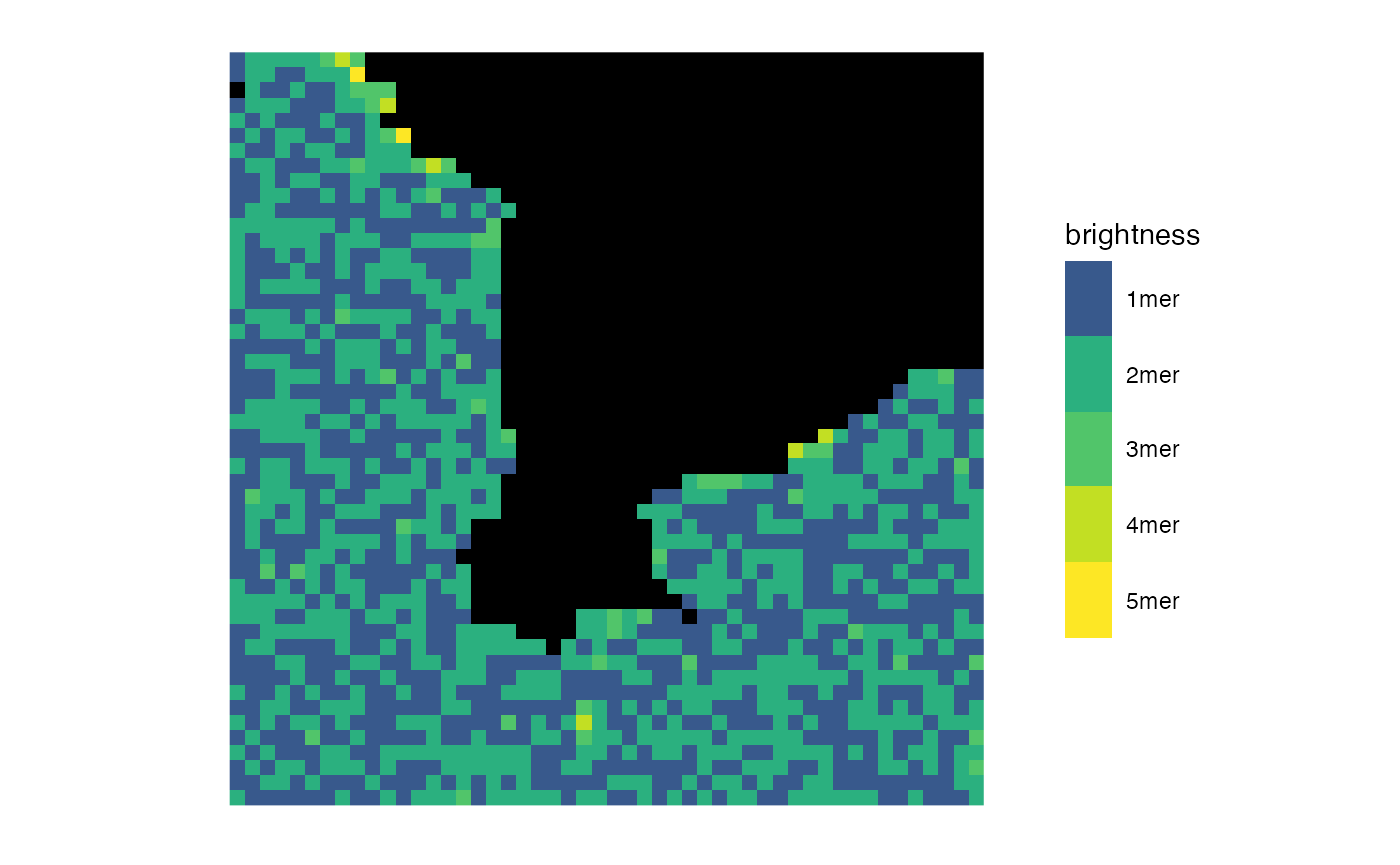
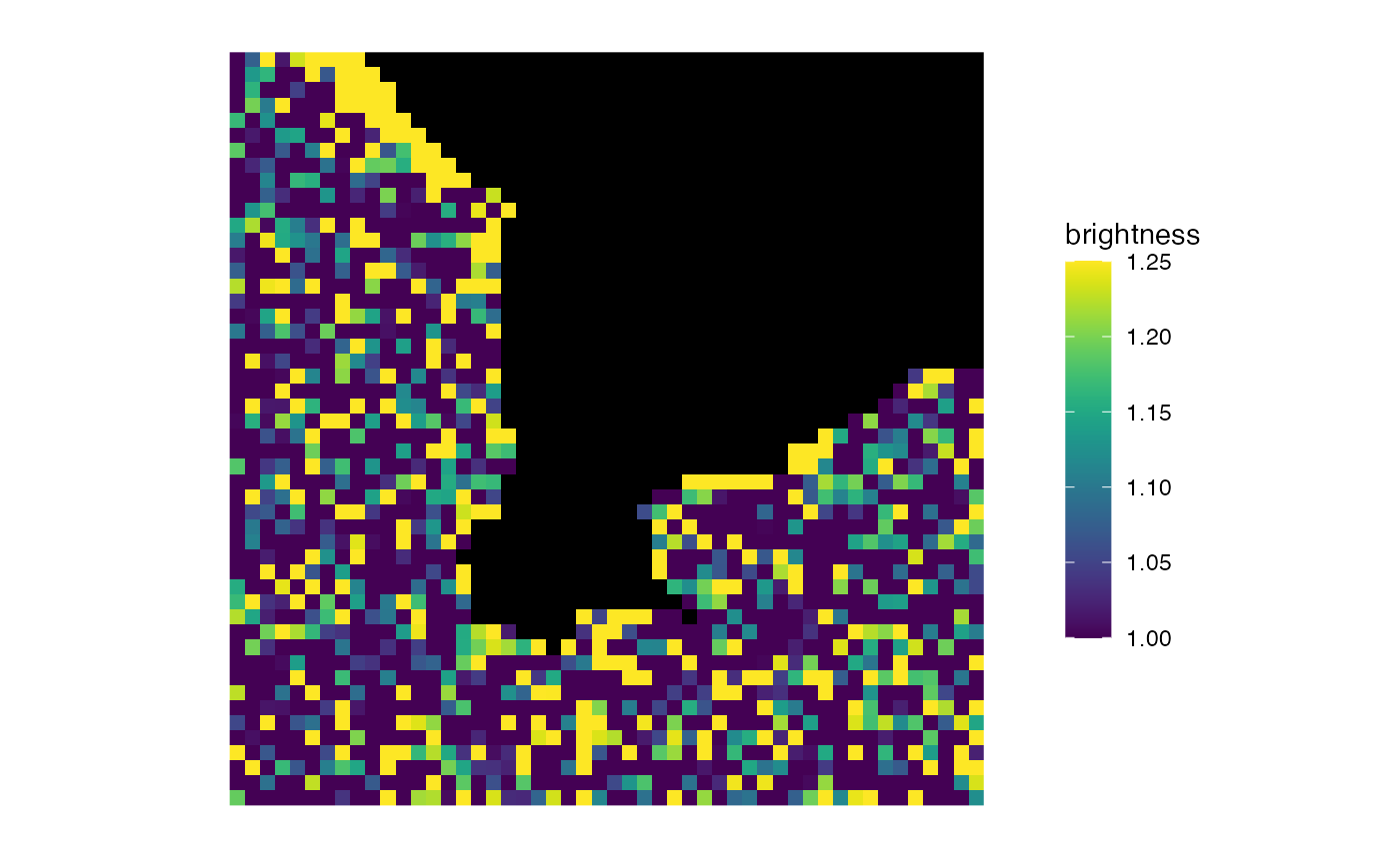
matrix_raster_plot(b,
  scale_name = "brightness",
  include_breaks = 1.25
)

# }