Chapter 1 Introduction

1.1 Fluorescence

Definition 1.1 Fluorescence is the emission of photons related to the process of relaxation for a given molecule from an electronically excited state (\(S_1\)) to the ground state (\(S_0\)).

These two electronic states (\(S_0\) and \(S_1\)) of a molecule are defined as the highest occupied molecular orbital (\(S_0\), HOMO) and the lowest unoccupied molecular orbital (\(S_1\), LUMO). Each electronic state has various associated vibrational states between which non-radiative transitions can occur. An electron can be excited from the ground state \(S_0\) into the higher energy excited state \(S_1\) by absorption of a photon of the appropriate energy. The electron will remain in the excited state (possibly undergoing non-radiative transitions through vibrational states) for a period of nanoseconds before relaxing to the lower energy ground state, losing energy by means of emitting a photon of that energy. This is shown by means of a Jablonski diagram (figure 1.1).

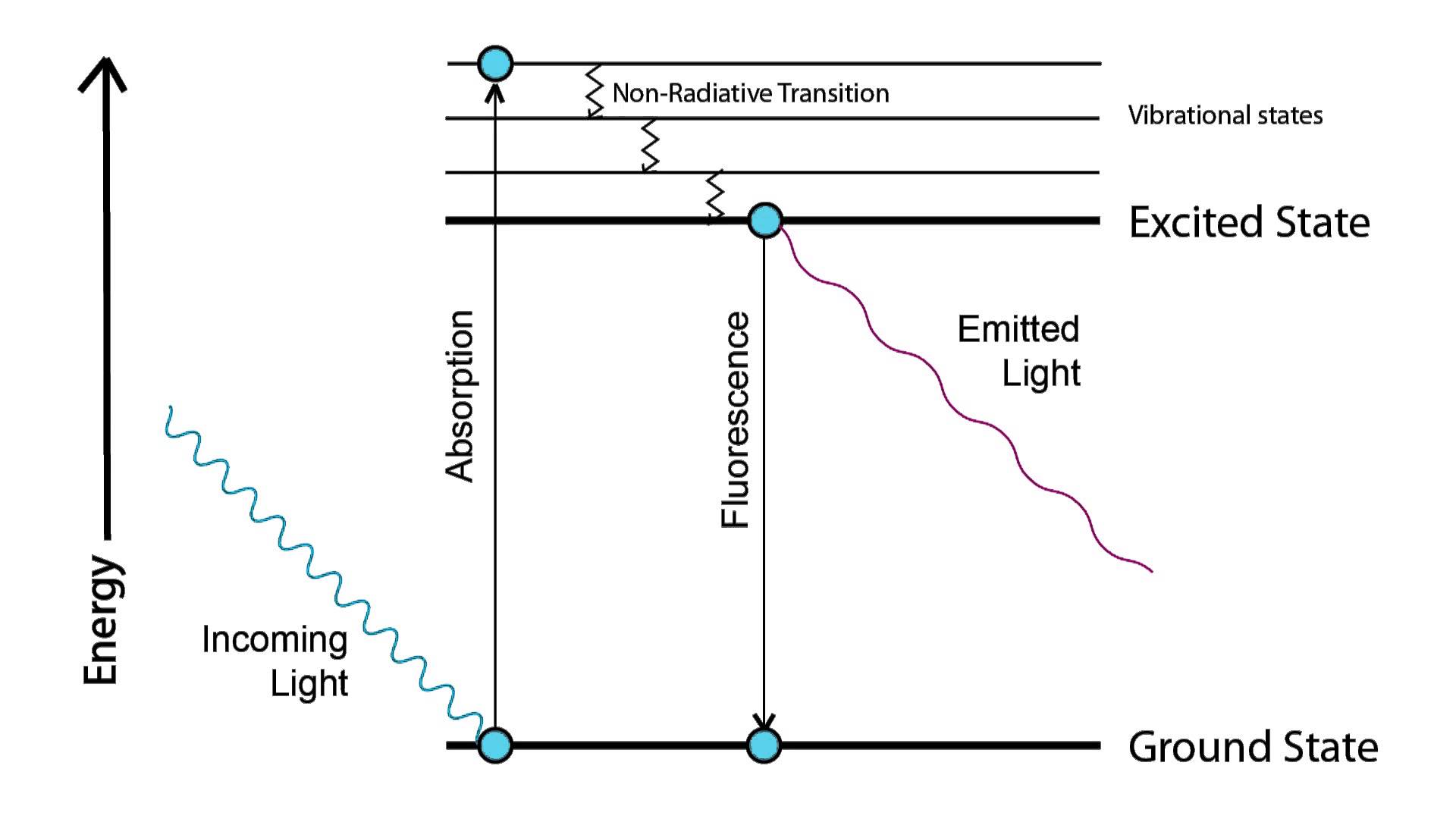
Figure 1.1: Jablonski diagram of the process of fluorescence. Absorption causes excitation, relaxation causes the emission of light.

Definition 1.2 The fluorescence lifetime of an electron is the amount of time it remains in the excited state before returning to the ground state.

Definition 1.3 A fluorophore is a fluorescent chemical compound that can re-emit light upon light excitation.

Fluorophores under constant excitation emit light one photon at a time according to Poisson statistics.

1.1.1 Phosphorescence

Definition 1.4 Excited electrons can undergo a forbidden transition into the triplet state \(T_1\), where they remain for a period of milliseconds before relaxing to the ground state with the emission of a photon. This is phosphorescence.

1.1.2 Photobleaching

In reality, an incident photon can break the fluorophore such that it is subsequently unable to emit light. A fluorophore to which this has happened is said to be photobleached.

1.2 Confocal light microscopy

All of the images used in my PhD were collected on a confocal microscope. This type of microscope guarantees that only in-focus light is collected at the detector. See figure 1.2.

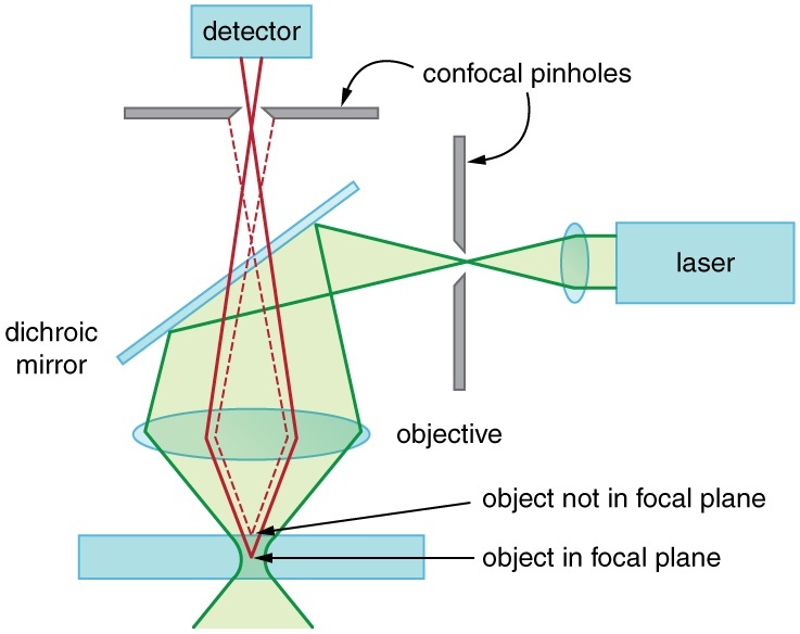
Figure 1.2: Confocal microscope light path showing how out of focus light does not make it to the detector.¹

Definition 1.5 The confocal volume is the in-focus volume within a sample that is efficiently detected using a system designed with confocal optics (FCSXpert 2018).

An image is acquired on a confocal microscope by scanning this apparatus across a sample, collecting one pixel at a time.

1.2.1 Detectors

There are many types of confocal microscope detectors. I will discuss the most common ones here. Most rely on the photoelectric effect (Albert Einstein 1905), a phenomenon whereby incident light upon a material causes electrons to dissociate from that material.

Definition 1.6 The quantum efficiency (QE) of a detector is the fraction of fluorescent signal that is reported by the detector.

1.2.1.1 Photon multiplier tubes

Photon multiplier tubes (PMTs) use the photoelectric effect. Dissociated electrons are accelerated through a potential difference towards a cathode where their accumulated kinetic energy is used to release more electrons. These are then accelerated in vacuum towards another cathode and so on for a predefined number of these accelerations until at last the electrons are discharged into an anode where the current is measured (Hammamatsu 2007); see figure 1.3. This current corresponds to the incident light intensity.

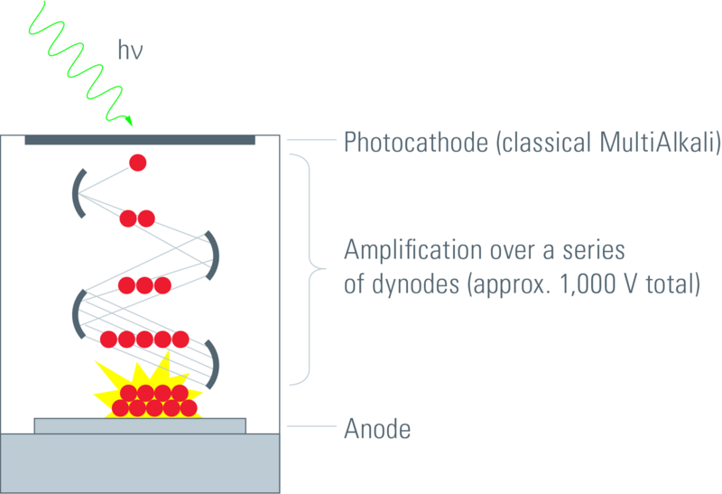
Figure 1.3: PMT detector setup. Electrons are dissociated by photons at the photocathode, accelerated towards various other cathodes where more and more are freed and then finally they arrive at the anode where the current is measured (Leica 2012).

The QE of standard PMTs is approximately 25% for blue-green light. This is because many incident photons on the multi-alkali material of regular PMT photocathodes fail to free any electrons. This problem gets worse at higher wavelengths where photons have lower energy. PMTs also suffer significantly from thermal noise (whereby dissociated electrons are created due to heat energy).

1.2.1.2 Avalanche photo-diodes

Definition 1.7 Avalanche multiplication in semiconductors occurs when free electrons which are moving in an electric field across the semiconductor collide with bound electrons, freeing them to move and indeed to free more bound electrons. This compounding increase in free electrons in the electric field leads to an increase in the electric current.

Avalanche photo-diodes (APDs) are semiconductors that exploit the photoelectric effect together with avalanche multiplication (the photoelectric effect starts the avalanche) to convert light into measurable electric current; see figure 1.4. They are somewhat analogous to PMTs, using the avalanche effect in place of the series of cathodes.

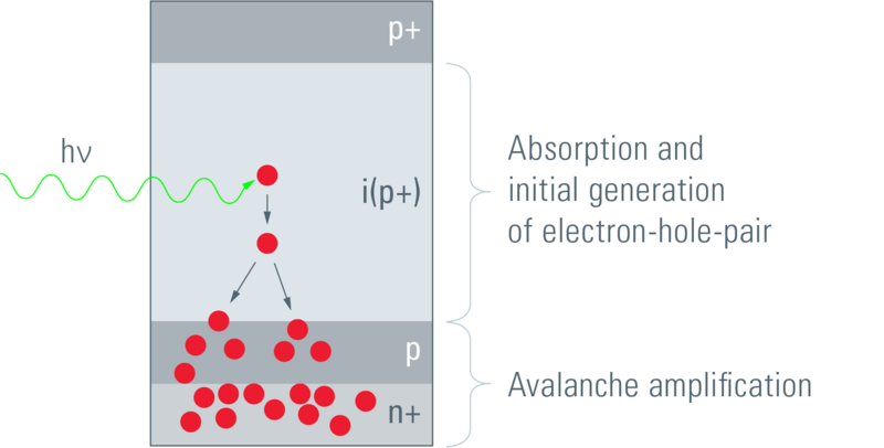
Figure 1.4: APD detector setup. The incident photon dissociates an electron. Given the electric field across the semiconductor, this electron is accelerated, initiating an avalanche (Leica 2012).

The QE of APDs can be as high as 45%, however their dynamic range is low and they can only function with low-intensity light. APDs are less prone to thermal noise than PMTs.

1.2.1.3 Hybrid detectors

APDs have better sensitivity and lower noise, however PMTs have a larger dynamic range. In hybrid detectors (HyDs), PMT and APD technology is combined to get the best of both worlds. With HyDs, photons are converted to electrons at the photocathode, then accelerated in vacuum towards a semiconductor where they initiate an electron avalanche. See figure 1.5. The difference between HyDs and APDs is this acceleration step.

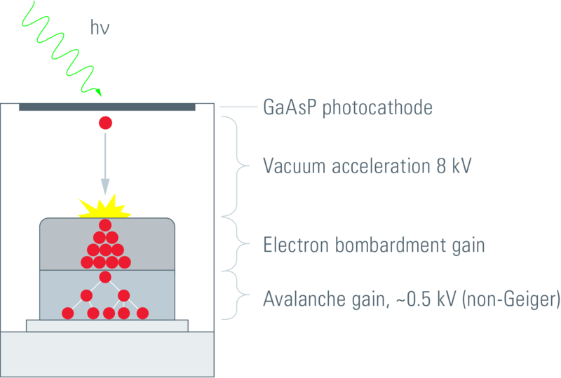
Figure 1.5: HyD detector setup. A photon dissociates an electron from the photocathode, this electron is then accelerated PMT-style towards an APD-style semiconductor setup, triggering an avalanche (Leica 2012).

HyDs with GaAsP (gallium arsenide phosphide) photocathodes achieve a quantum efficiency of up to 50% (Leica 2012). They also suffer least from detector afterpulsing, a phenomenon which can cause real signal pulses to be followed by a feedback pulse at a later time (Zhao et al. 2003).

With hybrid detectors, the electric current pulse caused by a photon striking the photocathode is strong (well above background) and sharp (the pulse is very short-lived). This means that it is easy to detect the arrival of single photons at the photocathode. This enables HyDs to have a photon-counting mode whereby the readout is in units of photons (not electron current). This is a much more physically relevant readout — given that we are interested in measuring fluorescence — which is very convenient for many biological applications, not least fluorescence fluctuation spectroscopy (FFS, discussed in section 1.5). For this reason, the HyD was the detector of choice for all of the acquisitions in my thesis.

Remark. Henceforth, intensity counts will be assumed to be in units of photons.

1.3 Intensity traces

Consider figure 1.6. A fluorophore enters the confocal volume, is excited there and emits photons which are collected by the detector. When the fluorophore is not in the confocal volume (start and end), no photons are detected. When the particle is in the confocal volume, photons it emits are collected at the detector. Different numbers of photons are collected per unit time (per ms here).

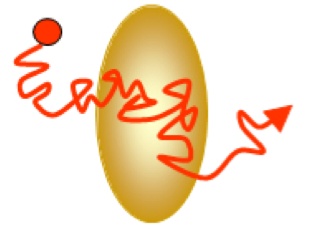
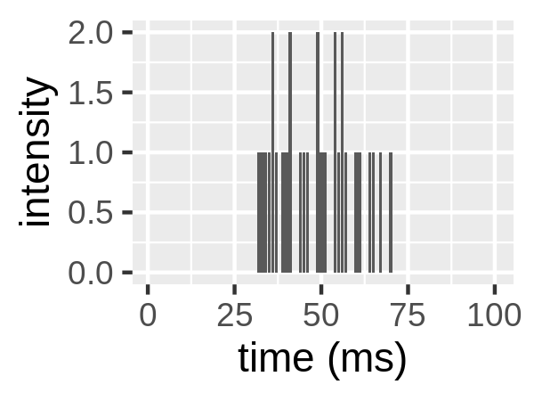
Figure 1.6: Left: a fluorophore diffusing through the confocal volume (Padilla-Parra 2009). Right: the intensity trace due to this fluorophore. This intensity trace has mean 0.3 and variance 0.31.

Definition 1.8 The time-series of intensity counts in a given pixel or image is referred to as its intensity trace.

1.4 Diffusion

Definition 1.9 Diffusion is the net movement of molecules or atoms from a region of high concentration (or high chemical potential) to a region of low concentration (or low chemical potential) as a result of random motion of the molecules or atoms.

Fick’s first law of diffusion relates the concentration to the diffusive flux, assuming a steady state. It describes how the flux goes from high to low concentration areas, with magnitude proportional to the concentration gradient. The law is:

\[\begin{equation} J = -D\frac{d\varphi}{dx} \tag{1.1} \end{equation}\]

where

• \(J\) is the diffusive flux
• \(D\) is the diffusion constant
• \(x\) is the position in space
• \(\varphi\) is the concentration at position \(x\).

Definition 1.10 Brownian motion is the random motion of particles suspended in a fluid resulting from their collision with the fast-moving molecules in the fluid (A. Einstein 1905).

Definition 1.11 In an ensemble of \(N\) particles, each of which occupies position \(x_i(t)\) at time \(t\), the mean squared displacement of the particles in the ensemble is

\[\begin{equation} \text{msd}(t) = \frac{1}{N}\sum_{i = 1}^N [x_i(t) - x_i(0)]^2 \tag{1.2} \end{equation}\]

For free Brownian motion in 1 dimension, the expected value of the MSD is \(\text{msd}(t) = 2Dt\), where \(D\) is the diffusion constant. For free Brownian motion in \(d\) dimensions, the expected value of the MSD is \(\text{msd}(t) = 2dDt\), reflecting the fact that free Brownian motion in \(d\) dimensions is one-dimensional free Brownian motion happening simultaneously and independently in each individual dimension.

These definitions are the formally correct ones. In biophysics, however, both of these processes (diffusion and Brownian motion) are most often referred to as diffusion. I will follow this convention.

1.4.1 Anomalous diffusion

Anomalous diffusion is a diffusion process whereby equation (1.2) no longer holds and the relationship between MSD and time becomes

\[\begin{equation} \text{msd}(t) = 2dDt^\alpha \tag{1.3} \end{equation}\]

where \(\alpha \neq 1\). \(\alpha > 1\) is known as superdiffusion (faster than normal) and \(\alpha < 1\) is known as subdiffusion (slower than normal).

1.4.2 Diffusion in the presence of barriers

If barriers to diffusion are present, neither equations (1.2) and (1.3) hold. The pair correlation function approach (section 1.6.3.1) can be used to image barriers to diffusion (Digman and Gratton 2009).

1.5 Fluorescence fluctuation spectroscopy

Broadly, fluorescence fluctuation spectroscopy (FFS) is the analysis of the intensity fluctuation of a fluorescence signal (Chen et al. 1999). This very often takes the form of moment analysis (Qian and Elson 1990). Briefly, moment analysis is an attempt to extract data from a distribution of values using its moments. The first moment of a distribution is its mean value, the second moment is its variance. The \(n\)^th moment of a random variable \(X\) with expected value \(E[X]=\mu\) for \(n>1\) is \(E[(X - \mu)^n]\).

Intensity traces can be viewed as distributions with moments. For example, the intensity trace in figure 1.6 has mean 0.3 and variance 0.31.

1.5.1 Number and brightness

Number and brightness (N&B, Digman et al. (2008)) is an FFS technique for quantifying the oligomeric states of fluorescently labelled proteins. What follows is a mathematical description of the technique.

Definition 1.12 An entity is a set of molecules which are chemically bound.

Definition 1.13 The brightness \(\epsilon\) of an entity is the mean number of photon detector counts it gives per unit time when in the illumination (confocal) volume.

For an image series where the \(i\)^th slice in the stack is the image acquired at time \(t = i\), for a given pixel position \((x, y)\), we define \(\langle I \rangle\) as the mean intensity of that pixel over the image series and \(\sigma^2\) as the variance in that intensity. Define \(n\) as the mean number of entities in the illumination volume corresponding to that pixel. Assuming that all entities are mobile, we have \[\begin{align} N &= \frac{\langle I \rangle^2}{\sigma^2} = \frac{\epsilon n}{1 + \epsilon} \tag{1.4} \\ B &= \frac{\sigma^2}{\langle I \rangle} = 1 + \epsilon \tag{1.5} \end{align}\] where \(N\) and \(B\) are referred to as the apparent number and apparent brightness respectively. This gives \[\begin{align} n &= \frac{\langle I \rangle^2}{\sigma^2 - \langle I \rangle} \tag{1.6} \\ \epsilon &= \frac{\sigma^2}{\langle I \rangle} - 1 \tag{1.7} \end{align}\]

These relations are derived using a moment analysis technique which was originally applied to molecules in solution (Qian and Elson 1990). With a scanning confocal microscope in analog mode, we must use three correction terms: 1. The proportionality constant \(S\), which is the conversion factor between photons detected and the number of counts returned by the analog electronics. 2. The offset (bias) due to the analog electronics in the level of the background. 3. The readout noise \(\sigma_0^2\) is the variance in this background signal (Dalal et al. 2008). Then, if all entities are mobile, we have

\[\begin{align} N &= \frac{(\langle I \rangle - \text{ offset})^2}{\sigma^2 - \sigma_0^2} = \frac{\epsilon n}{1 + \epsilon} \tag{1.8} \\ B &= \frac{\sigma^2 - \sigma_0^2}{\langle I \rangle - \text{ offset}} = S(1 + \epsilon) \tag{1.9} \end{align}\] \[\begin{align} n &= \frac{(\langle I \rangle - \text{ offset})^2}{\sigma^2 - \sigma_0^2 - S(\langle I \rangle - \text{ offset})} \tag{1.10} \\ \epsilon &= \frac{\sigma^2 - \sigma_0^2}{S(\langle I \rangle - \text{ offset})} - 1 \tag{1.11} \end{align}\]

— Nolan, Iliopoulou, et al. (2017)²

The quantity \(\epsilon\) is a relative measure of oligomeric state. That is, \(\epsilon\) will be twice as big for dimers as it is for monomers, three times as big for trimers as it is for monomers and so on.

The way that N&B experiments to determine unknown oligomeric states are generally done is as follows:

1. For a given laser power and fluorophore with a system where all entities are known to be monomeric, measure the brightness \(\epsilon\). Call this \(\epsilon_\text{monomer}\).
2. With the same laser power and fluorophore but now with a system where the oligomeric state is unknown, measure the brightness \(\epsilon\) again. Call this \(\epsilon_\text{unknown}\).
3. The unknown oligomeric state is equal to \(\epsilon_\text{unknown} / \epsilon_\text{monomer}\).

Number and brightness has specific pixel dwell-time and frame rate requirements. These were first articulated in my 2017 review of N&B (Nolan, Iliopoulou, et al. 2017).

Definition 1.14 The pixel dwell time \(t_\text{dwell}\) of a scanning confocal microscope is the amount of time it spends collecting photons at each given pixel before moving on to the next pixel.

It is essential that the pixel dwell time is the same for each pixel, particularly for FFS. This is something that must be carefully verified on each instrument. This can be done with a chroma-slide. The photon counts measured from a chroma-slide should follow a Poisson distribution. If instead the distribution is super-Poissonian (has a greater variance than its mean), this is indicative of a non-constant dwell-time.

Definition 1.15 The frame time \(t_\text{frame}\) of a scanning confocal microscope is the amount of time it takes to acquire the data for all of the pixels in a whole frame. That is the length of time from the start of detection of photons from the first pixel to the end of detection of photons from the last pixel.

Definition 1.16 The mean residence time \(\tau_D\) of a particle in the confocal volume is the average length of time that a particle that enters the confocal volume resides in that volume before exiting.

The requirement is \(t_\text{dwell} \ll \tau_D \ll t_\text{frame}\). This ensures that:

1. When acquiring photons at a given pixel, the underlying configuration of entities is constant (there’s not enough time for the entities to move and change their configuration).
2. When the scanner returns to a given pixel (one frame time later), the underlying configuration has changed totally since the last time the scanner was at this pixel (because so much time has passed, all of the diffusing entities have moved a lot in the meantime).

Both of these points are implicitly assumed in the derivation of the N&B equations so it is essential to get these acquisition parameters right. This is discussed at length in Nolan, Iliopoulou, et al. (2017).

An important property of N&B is that if all fluorescent particles are immobile, then \(B = 1\). This is because photon emission from stationary sources happens according to a Poisson distribution. Poisson distributions have variance equal to mean, this implies \(\sigma^2\) = \(\langle I \rangle\) which gives \(B = \frac{\sigma^2}{\langle I \rangle} = 1\).

The N&B technique is fraught with technical difficulties. Principal of these is the problem of photobleaching. Most of my PhD focused on corrections for photobleaching. This is discussed in chapter 3.

1.6 Fluorescence correlation spectroscopy

Fluorescence correlation spectroscopy (FCS) is the correlation analysis of fluorescence intensity fluctuations. For this reason, FCS can be described as a subfield of FFS (Jameson, Ross, and Albanesi 2009). In practice, FFS is mostly used to refer to the non-FCS parts of the whole FFS field. I will follow that convention.

First, let us introduce some concepts from statistics. Let \(X\) and \(Y\) be random variables manifested in observations \(\{x_1, x_2, \ldots, x_T\}\) and \(\{x_1, x_2, \ldots, x_T\}\) taken at times \(t = 1, 2, \ldots, T\). Let \(X\) and \(Y\) have expected values \(\mu_X\) and \(\mu_Y\) and variances \(\sigma^2_x\) and \(\sigma^2_Y\).

Definition 1.17 (statistics) The correlation between random variables \(X\) and \(Y\) is \[\begin{equation} \text{corr}(X, Y) = \frac{E[(X - \mu_X)(Y - \mu_Y)]}{\sigma_X \sigma_Y} \tag{1.12} \end{equation}\] where \(E\) is the expectation operator.

Definition 1.18 (statistics) Autocorrelation \(G(X; \tau)\), is the correlation of a signal \(X\) with a delayed copy of itself as a function of the delay \(\tau\).

Statisticians define this in two different ways:

\[\begin{equation} G_1(X; \tau) = \frac{E[(X_t - \mu_X)(X_{t + \tau} - \mu_X)]}{\sigma^2_X} \tag{1.13} \end{equation}\] \[\begin{equation} G_2(X; \tau) = \frac{\sum_{t = \tau + 1}^T (x_t - \mu_x)(x_{t - \tau} - \mu_x)}{\sum_{t = 1}^T [(x_t -\mu_x)^2]} \tag{1.14} \end{equation}\]

The relationship between \(G_1\) and \(G_2\) is

\[\begin{equation} G_2(X; \tau) = \frac{T - \tau}{T - 1} \times G_1(X; \tau) \tag{1.15} \end{equation}\]

Remark. Above, I have labelled these \(G_1\) and \(G_2\) to distinguish the definitions, but elsewhere people will just use \(G\) (or something else) and it will be up to you—the reader—to figure out which one is being used. \(G_2\) is often used in the statistics field of time-series analysis. A modified version of \(G_1\) is used in FCS (this modified version is defined below).

Definition 1.19 (statistics) The cross-correlation of two series is the correlation of one with a delayed copy of the other as a function of the delay. \[\begin{equation} \text{crosscorr}(X, Y; \tau) = \text{corr}(X_t, Y_{t + \tau}) = \frac{E[(X_t - \mu_X)(Y_{t + \tau} - \mu_Y)]}{\sigma_X \sigma_Y} \tag{1.16} \end{equation}\]

For the purposes of FCS, these quantities were redefined as follows.

Definition 1.20 (FCS) The correlation between two random variables \(X\) and \(Y\) with expected values \(\mu_X\) and \(\mu_Y\) and standard deviations \(\sigma_X\) and \(\sigma_Y\) is \[\begin{equation} \text{corr}(X, Y) = \frac{E[(X - \mu_X)(Y - \mu_Y)]}{\mu_X \mu_Y} \tag{1.17} \end{equation}\] where \(E\) is the expectation operator.

Definition 1.21 (FCS) Autocorrelation \(G(X; \tau)\), is the correlation of a signal \(X\) with a delayed copy of itself as a function of the delay \(\tau\). \[\begin{equation} G(X; \tau) = \text{corr}(X_t, X_{t + \tau}) = \frac{E[(X_t - \mu_X)(X_{t + \tau} - \mu_X)]}{\mu^2_X} \tag{1.18} \end{equation}\]

Definition 1.22 (FCS) The cross-correlation of two series is the correlation of one with a delayed copy of the other as a function of the delay. \[\begin{equation} \text{crosscorr}(X, Y; \tau) = \text{corr}(X_t, Y_{t + \tau}) = \frac{E[(X_t - \mu_X)(Y_{t + \tau} - \mu_Y)]}{\mu_X \mu_Y} \tag{1.19} \end{equation}\]

The reason for these redefinitions (which just involve replacing standard deviations with means in the denominators of each expression) is that with the FCS definition, the autocorrelation has the nice property that for normal diffusion

\[\begin{equation} G(X; 0) = \frac{1}{n} \tag{1.20} \end{equation}\]

where \(n\) is the mean number of fluorescent particles in the focal volume. The convenience of the statistics definitions is that there, correlations are guaranteed to be in \([-1, 1]\), with \(0\) representing no correlation, \(1\) perfect positive correlation and \(-1\) perfect negative correlation; this is lost with the FCS definitions: 0 still represents no correlation, but correlation values are no longer bounded, so the ideas of perfect correlation are lost.

I felt it necessary to provide these definitions for two reasons:

1. It is important for people from the fields of FCS and pure mathematics/statistics to know that they have different definitions for the same thing.
2. In FCS, it’s very common for people to mistake correlation for cross-correlation. This is unfortunate, but knowing about this common mistake is essential for navigating the field in a sensible manner. It seems that when people in the FCS field correlate the signals from two separate channels, they use the term cross-correlation, even though they’re only using correlation. I think the idea of working across two or more channels (and ideas such as cross-talk) leads to this confusion.

Remark. Henceforth, the FCS defintions of these quantities will be assumed.

1.6.1 Correlation

Co-diffusing fluorophores of different colours will necessarily induce positive correlation between the intensity traces of these two colour channels because co-diffusion means that presence of one fluorophore necessarily implies presence of the other fluorophore. Hence, correlation may be used as a measure of co-diffusion, and co-diffusion is often interpreted as interaction (the simplest explanation for co-diffusion is that the co-diffusing entities are somehow stuck together). This idea forms the basis of much of FCS.

This does not hold for immobile particles. Immobile particles are not diffusing, so it doesn’t make sense to employ a measure of diffusion.

Bleed-through of photons from one channel to another will induce artefactual correlation between the intensities of the two channels. Alternating laser excitation (ALEX, Kapanidis et al. (2005)) can be used to eliminate bleed through; however when using ALEX it is important to bear in mind that the two channels are no longer being acquired simultaneously. This is of particular importance for FCS. However if the instrument can go fast enough (with a laser alternation time much less than the residence time of the diffusing entities), this problem is negligible.

If the density of fluorophores under observation is too high, correlation can be practically impossible to measure. For example, the difference between 1 and 0 is much easier to detect than the difference between 11 and 10. At high density, relative differences are lower and hence harder to detect.

1.6.2 Autocorrelation

As mentioned already, the autocorrelation function (ACF) can be used to count the number of particles in the confocal volume. It can also be used to measure diffusion coefficients. The ACF is not used in my PhD.

1.6.3 Cross-correlation

The cross-correlation of intensity traces from nearby pixels can be used to measure the velocity of the movement of the labelled particles between these two pixels (Hebert, Costantino, and Wiseman 2005).

1.6.3.1 Pair correlation function

The phrase pair correlation function³ was coined for this idea of cross-correlating intensity traces from nearby pixels. The PCF was used to image barriers to diffusion (Digman and Gratton 2009) using the idea that the spatiotemporal correlation caused by particles moving from one place to another will not be present for positions \(p_1\) and \(p_2\) if they are on opposite sides of a barrier, because the barrier prevents travel from \(p_1\) to \(p_2\). It has also been used to calculate the velocities of diffusing entities at each pixel in an image. The collection of these velocities at each pixel is known as a diffusion tensor (Rienzo et al. 2016). This approach is similar to that of Hebert, Costantino, and Wiseman (2005).

1.6.4 Cross-correlated brightness

Cross-correlated brightness (Digman et al. 2009) molds the correlation idea (section 1.6.1) into the framework of N&B. Cross-correlated brightness isn’t really a brightness at all, it’s just a measure of correlation.

Suppose there are two channels with intensities \(I_1\) and \(I_2\).

Definition 1.23 (cross-variance) \[\begin{equation} \sigma^2_\text{cc} = E[(I_2 - \langle I_1 \rangle)(I_2 - \langle I_2 \rangle)] \tag{1.21} \end{equation}\]

Definition 1.24 (cross-correlated brightness) \[\begin{equation} B_\text{cc} = \frac{\sigma^2_\text{cc}}{\sqrt{\langle I_1 \rangle \langle I_2 \rangle}} \tag{1.22} \end{equation}\]

\(B_\text{cc}\) is related to \(\text{corr}(I_1, I_2)\) by \[\begin{equation} B_\text{cc} = \sqrt{\langle I_1 \rangle \langle I_2 \rangle} \times \text{corr}(I_1, I_2) \tag{1.23} \end{equation}\]

This means that \(B_\text{cc}\) is just a scaled version of correlation. The need for this redefinition is unclear (but it is no harm). It does make the formula look like the brightness formula (1.5), but no such oligomeric state information can be gleaned from \(B_\text{cc}\). It is merely useful as a relative measure of interaction: higher \(B_\text{cc}\) means more interaction, lower \(B_\text{cc}\) means less interaction. It is commonly used to identify interactions. Then, conventional N&B performed on each of the channels (1 and 2) can be used to measure the stoichiometry of the interaction.

Remark. Since cross-correlated brightness uses correlation but not cross-correlation, it is a prime example of the confusing naming that pervades FCS. It should be called correlated brightness. Rather than rename it, I will continue to refer to it as cross-correlated brightness.

1.7 Applications of FCS and FFS

FCS and FFS have been used in thousands of research projects. Here I number but a few for the sake of interest and to give biological context to these techniques.

Number and brightness (the prominent imaging FFS technique) has been used to:

• characterize the state of DNA aggregation in live cells (Mieruszynski et al. 2015)
• measure the stoichiometry of scaffold complexes in live neurons (Moutin et al. 2014)
• quantify interactions in gene expression networks (Declerck and Royer 2013)
• measure the oligomeric state of the dynamin-2 protein at the HIV-1 fusion pore (Jones et al. 2017)
• measure the stoichiometry of the interaction of HIV-1 with its receptor and co-receptor over time in the pre-fusion process (Iliopoulou et al. 2018)

FCS has been used to:

• reveal structural and functional properties of promyelocytic leukemia nuclear bodies (Hoischen et al. 2018)
• demonstrate that HIV-1 evades antibody-dependent phagocytosis (Gach et al. 2017)
• determine the size of nanodomains (Fenz, Smith, and Monzel 2017)
• perform chromatographic measurements (Kisley and Landes 2014)
• quantify interactions of membrane proteins (Ly et al. 2014)

References

Chen, Y., J. D. Muller, K. M. Berland, and E. Gratton. 1999. “Fluorescence fluctuation spectroscopy.” Methods 19 (2): 234–52. doi:10.1006/meth.1999.0854.

Dalal, R. B., M. A. Digman, A. F. Horwitz, V. Vetri, and E. Gratton. 2008. “Determination of particle number and brightness using a laser scanning confocal microscope operating in the analog mode.” Microsc. Res. Tech. 71 (1): 69–81. doi:10.1002/jemt.20526.

Declerck, Nathalie, and Catherine A. Royer. 2013. “Interactions in Gene Expression Networks Studied by Two-Photon Fluorescence Fluctuation Spectroscopy.” In Methods in Enzymology, 203–30. Elsevier. doi:10.1016/b978-0-12-405539-1.00007-5.

Digman, M. A., and E. Gratton. 2009. “Imaging barriers to diffusion by pair correlation functions.” Biophys. J. 97 (2): 665–73. doi:10.1016/j.bpj.2009.04.048.

Digman, M. A., R. Dalal, A. F. Horwitz, and E. Gratton. 2008. “Mapping the number of molecules and brightness in the laser scanning microscope.” Biophys. J. 94 (6): 2320–32. doi:10.1529/biophysj.107.114645.

Digman, M. A., P. W. Wiseman, C. Choi, Alan R. Horwitz, and E. Gratton. 2009. “Stoichiometry of Molecular Complexes at Adhesions in Living Cells.” Proceedings of the National Academy of Sciences 106 (7). National Academy of Sciences: 2170–5. doi:10.1073/pnas.0806036106.

Einstein, A. 1905. “Über Die von Der Molekularkinetischen Theorie Der Wärme Geforderte Bewegung von in Ruhenden Flüssigkeiten Suspendierten Teilchen.” Annalen Der Physik 322 (8). Wiley: 549–60. doi:10.1002/andp.19053220806.

Einstein, Albert. 1905. “Concerning an Heuristic Point of View Toward the Emission and Transformation of Light.” Annalen Der Physik 17: 132–48.

FCSXpert. 2018. “What Is the Confocal Volume?” Sensor Technologies LLC. http://www.fcsxpert.com/classroom/theory/what-is-confocal-volume.html.

Fenz, Susanne F., Ana-Sunčana Smith, and Cornelia Monzel. 2017. “Measuring the Invisible: Determining the Size of Growing Nanodomains Using the Inverse FCS.” Biophysical Journal 112 (11). Elsevier BV: 2245–6. doi:10.1016/j.bpj.2017.04.014.

Gach, Johannes S., Margaux Bouzin, Marcus P. Wong, Veronika Chromikova, Andrea Gorlani, Kuan-Ting Yu, Brijesh Sharma, Enrico Gratton, and Donald N. Forthal. 2017. “Human Immunodeficiency Virus Type-1 (HIV-1) Evades Antibody-Dependent Phagocytosis.” Edited by Alexandra Trkola. PLOS Pathogens 13 (12). Public Library of Science (PLoS): e1006793. doi:10.1371/journal.ppat.1006793.

Hammamatsu. 2007. “Photomultiplier Tubes: Basics and Applications.” Hammamatsu. https://www.hamamatsu.com/resources/pdf/etd/PMT_handbook_v3aE.pdf.

Hebert, B., S. Costantino, and P. W. Wiseman. 2005. “Spatiotemporal image correlation spectroscopy (STICS) theory, verification, and application to protein velocity mapping in living CHO cells.” Biophys. J. 88 (5): 3601–14. doi:10.1529/biophysj.104.054874.

Hoischen, Christian, Shamci Monajembashi, Klaus Weisshart, and Peter Hemmerich. 2018. “Multimodal Light Microscopy Approaches to Reveal Structural and Functional Properties of Promyelocytic Leukemia Nuclear Bodies.” Frontiers in Oncology 8 (May). Frontiers Media SA. doi:10.3389/fonc.2018.00125.

Iliopoulou, Maro, Rory Nolan, Luis Alvarez, Yasunori Watanabe, Charles A. Coomer, G. Maria Jakobsdottir, Thomas A. Bowden, and Sergi Padilla-Parra. 2018. “A dynamic three step mechanism drives the HIV-1 prefusion reaction.” Nat. Struct. Mol. Biol. 25 (9). doi:10.1038/s41594-018-0113-x.

Jameson, D. M., J. A. Ross, and J. P. Albanesi. 2009. “Fluorescence fluctuation spectroscopy: ushering in a new age of enlightenment for cellular dynamics.” Biophys Rev 1 (3): 105–18. doi:10.1007/s12551-009-0013-8.

Jones, Daniel M, Luis A Alvarez, Rory Nolan, Margarita Ferriz, Raquel Sainz Urruela, Xènia Massana-Muñoz, Hila Novak-Kotzer, Michael L Dustin, and Sergi Padilla-Parra. 2017. “Dynamin-2 Stabilizes the Hiv-1 Fusion Pore with a Low Oligomeric State.” Cell Reports 18 (2). Elsevier: 443–53. doi:10.1016/j.celrep.2016.12.032.

Kapanidis, Achillefs N., Ted A. Laurence, Nam Ki Lee, Emmanuel Margeat, Xiangxu Kong, and Shimon Weiss. 2005. “Alternating-Laser Excitation of Single Molecules.” Accounts of Chemical Research 38 (7). American Chemical Society (ACS): 523–33. doi:10.1021/ar0401348.

Kisley, Lydia, and Christy F. Landes. 2014. “Molecular Approaches to Chromatography Using Single Molecule Spectroscopy.” Analytical Chemistry 87 (1). American Chemical Society (ACS): 83–98. doi:10.1021/ac5039225.

Leica. 2012. “Sensors for True Confocal Scanning.” Leica Microsystems. https://www.leica-microsystems.com/science-lab/sensors-for-true-confocal-scanning/.

Ly, Sonny, Feliza Bourguet, Nicholas O. Fischer, Edmond Y. Lau, Matthew A. Coleman, and Ted A. Laurence. 2014. “Quantifying Interactions of a Membrane Protein Embedded in a Lipid Nanodisc Using Fluorescence Correlation Spectroscopy.” Biophysical Journal 106 (2). Elsevier BV: L05–L08. doi:10.1016/j.bpj.2013.12.014.

Mieruszynski, Stephen, Candida Briggs, Michelle A. Digman, Enrico Gratton, and Mark R Jones. 2015. “Live Cell Characterization of DNA Aggregation Delivered Through Lipofection.” Scientific Reports 5 (1). Springer Nature. doi:10.1038/srep10528.

Moutin, E., V. Compan, F. Raynaud, C. Clerte, N. Bouquier, G. Labesse, M. L. Ferguson, L. Fagni, C. A. Royer, and J. Perroy. 2014. “The Stoichiometry of Scaffold Complexes in Living Neurons - DLC2 Functions as a Dimerization Engine for GKAP.” Journal of Cell Science 127 (16). The Company of Biologists: 3451–62. doi:10.1242/jcs.145748.

Nolan, Rory, Maro Iliopoulou, Luis Alvarez, and Sergi Padilla-Parra. 2017. “Detecting Protein Aggregation and Interaction in Live Cells: A Guide to Number and Brightness.” Methods. doi:10.1016/j.ymeth.2017.12.001.

Padilla-Parra, Sergi. 2009. “Developpments Methodologiques Pour La Quantification Des Interactions Proteiques En Cellules Vivantes Par Microscopie de Fluorescence.” PhD thesis, Universite Paris Diderot.

Qian, H., and E. L. Elson. 1990. “Distribution of molecular aggregation by analysis of fluctuation moments.” Proc. Natl. Acad. Sci. U.S.A. 87 (14): 5479–83. doi:10.1073/pnas.87.14.5479.

Rienzo, Carmine Di, Francesco Cardarelli, Mariagrazia Di Luca, Fabio Beltram, and Enrico Gratton. 2016. “Diffusion Tensor Analysis by Two-Dimensional Pair Correlation of Fluorescence Fluctuations in Cells.” Biophysical Journal 111 (4). Elsevier BV: 841–51. doi:10.1016/j.bpj.2016.07.005.

Zhao, M., L. Jin, B. Chen, Y. Ding, H. Ma, and D. Chen. 2003. “Afterpulsing and its correction in fluorescence correlation spectroscopy experiments.” Appl Opt 42 (19): 4031–6.

---

1. Image courtesy of Quora: https://www.quora.com/How-does-confocal-microscopy-work↩

2. This is a formulation of N&B that I wrote in a 2017 review of the technique.↩

3. This was needless, it could just be called cross-correlation function but for the confusion about the term cross-correlation in the FCS field.↩