Chapter 3 Photobleaching Correction

3.1 Introduction to photobleaching

In the ideal case, an incident photon of appropriate wavelength is absorbed by a fluorophore, promoting the fluorophore to an excited state; subsequently, the fluorophore relaxes down to its ground state by emitting a photon. In reality, it is possible that the incident photon can break the fluorophore with the result that it will no longer emit light. This breaking is referred to as photobleaching (or bleaching for short). Bleaching causes a diminution in the number of effective fluorophores, which is a direct cause of a loss of fluorescent signal.

Many quantitative methods in fields such as fluorescence fluctuation spectroscopy (FFS) and fluorescence correlation spectroscopy (FCS) implicitly assume that there is no bleaching in the data. Hence, data (image series) with significant levels of photobleaching must be corrected prior to the application of equations and algorithms in these fields. A main focus of this thesis is on how to correct fluorescent image series for the effects of bleaching, given that bleaching does occur. There is no attempt to understand why and/or how photobleaching occurs.

Remark. All of the current literature mentions bleaching correction as being purely for correcting the problem of non-stationary mean (NSM), neglecting the problem of non-stationary variance (NSV). Figure 3.5 shows that NSM and NSV go hand-in-hand. Correction for NSM is referred to as trend removal or detrending. Hence, the terms detrending and bleaching correction have come to be used interchangeably. I will follow this convention and use the term detrending from now on to mean correction for NSM and possibly also NSV. Starting at section 3.3, the focus is on correcting for NSM. Discussion of correction for NSV starts in section 3.7.

3.2 The effects of bleaching in FCS and FFS

We simulate two image series with 500 frames, 64x64 pixels per frame (pixel size 1 $\mu$m), each with 100,000 diffusing ($D = 100~\mu\text{m}^2/\text{s}$) fluorescent particles which are uniformly distributed at the beginning. In the first image series (img1), these have brightness $\epsilon = 4$ and in the second (img2) they have brightness $\epsilon = 7$. See figure 3.1. We bleach these by 15% and 20% to create img1_bleached and img2_bleached respectively.

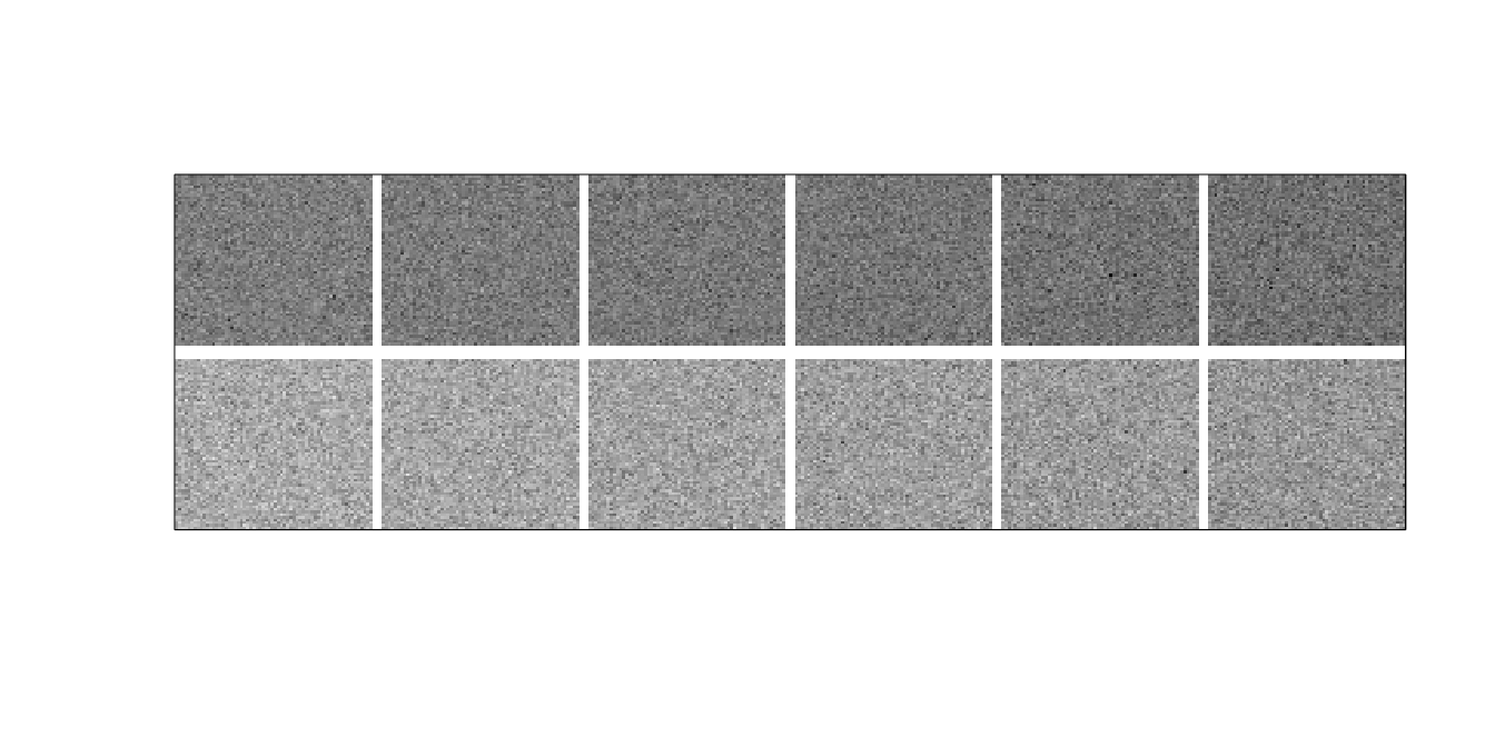
$Frames 1, 100, 200, 300, 400 and 500 from simulated image series. $\epsilon = 4$ (top) and $\epsilon = 7$ (bottom) with 15% (top) and 20% (bottom) bleaching.$

Figure 3.1: Frames 1, 100, 200, 300, 400 and 500 from simulated image series. $\epsilon = 4$ (top) and $\epsilon = 7$ (bottom) with 15% (top) and 20% (bottom) bleaching.

It may not be obvious that these image series are subject to bleaching from figure 3.1, but we can see it more clearly in figure 3.2.

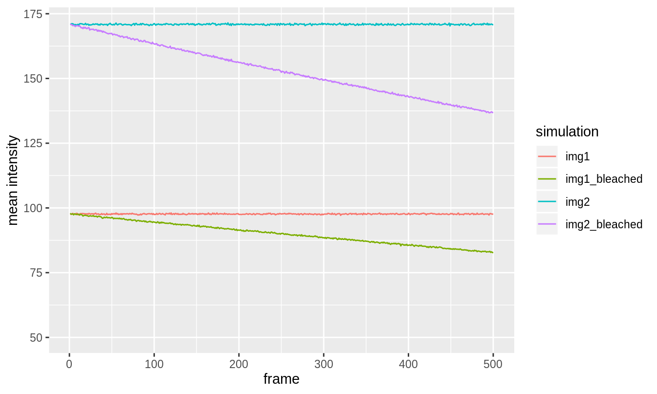
Mean intensity profiles of the simulated image series with and without bleaching. Simulation 1 was bleached by 15% and simulation 2 by 20%. The bleaching is such that the mean intensity decreases according to a single exponential decay (even though it looks quite linear).

Figure 3.2: Mean intensity profiles of the simulated image series with and without bleaching. Simulation 1 was bleached by 15% and simulation 2 by 20%. The bleaching is such that the mean intensity decreases according to a single exponential decay (even though it looks quite linear).

3.2.1 FCS

The unrelated images img1 and img2 have a tiny median cross-correlated brightness of $B_\text{cc} = 0.0036$, signifying no significant correlation, as one would expect. However, the bleached images img1_bleached and img2_bleached have a significant $B_\text{cc} = 0.3686$. This shows that bleaching is introducing correlation between otherwise unrelated images. Since correlation is used as a proxy for hetero-interaction, bleaching can make it appear as though there is interaction when in fact there is not.

3.2.1.1 Why does bleaching introduce correlation

Let’s take another look at the formula for correlation:

Definition 3.1 (FCS) The correlation between two random variables $X$ and $Y$ with expected values $\mu_X$ and $\mu_Y$ and standard deviations $\sigma_X$ and $\sigma_Y$ is \[\begin{equation} \text{corr}(X, Y) = \frac{E[(X - \mu_X)(Y - \mu_Y)]}{\mu_X \mu_Y} \tag{3.1} \end{equation}\]

So correlation is answering the question: Do $X$ and $Y$ deviate from their mean at the same time and in the same or opposite direction? If there is no pattern in their deviations from mean, then the correlation will be zero. If they deviate from their means in the same direction at the same time, there will be a positive correlation; if they deviate from their means in the opposite direction at the same time, there will be a negative correlation. Correlation is all about measuring whether deviation from mean in two different series is synchronised or not.

Let’s create two unrelated intensity traces $X$ and $Y$, both of length 500. $X$ will be Poisson($\lambda = 50$) and $Y$ will be Poisson($\lambda = 30$).

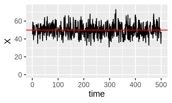
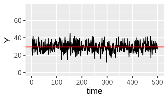
$Unrelated intensity traces $X$ and $Y$ with their means in red.$ $Unrelated intensity traces $X$ and $Y$ with their means in red.$

Figure 3.3: Unrelated intensity traces $X$ and $Y$ with their means in red.

There’s no pattern in how $X$ and $Y$ deviate from their means, indeed a Pearson correlation test of $X$ and $Y$ returns an insignificant $p$-value of 0.28.

Now let’s bleach them both by 90%.

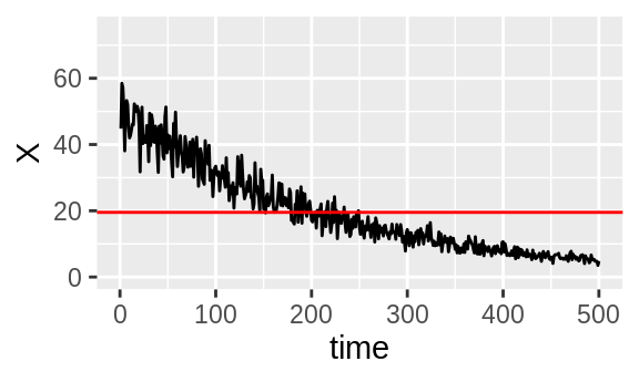
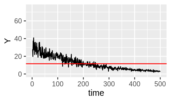
$Unrelated intensity traces $X$ and $Y$ with their means in red.$ $Unrelated intensity traces $X$ and $Y$ with their means in red.$

Figure 3.4: Unrelated intensity traces $X$ and $Y$ with their means in red.

Now, there is visible correlation. At the start of $X$ and $Y$, both are consistently above their mean and at the end, both are consistently below. They are simultaneously above and below respectively, so there will be positive correlation. This is backed up by a Pearson correlation test which returns a significant $p$-value of less than $10^{-200}$.

Remark. Bleaching also introduces autocorrelation for the same reason. The series $X$ had no autocorrelation before bleaching ($p$ = 0.23), whereas after bleaching, $X$ has significant autocorrelation ($p < 10^{-200}$).

3.2.2 FFS

Definition 3.2 (median mean pixel intensity) The median mean pixel intensity of an image series is found by taking the mean intensity of each pixel in the image series and then taking the median of those means. It can be thought of as a summary statistic for the pixel intensity of the image series.

Definition 3.3 (median pixel intensity variance) The median pixel intensity variance of an image series is found by taking the variance in the intensity of each pixel in the image series and then taking the median of those variances. It can be thought of as a summary statistic for the variance in the pixel intensity of the image series.

In FFS, one is always interested in the mean and variance of pixel values. img1 has a median mean pixel intensity of 98 and a median pixel intensity variance of 487. The mean brightness is $\epsilon = 3.9959$ (very close to 4, as expected since the image series was simulated with brightness $\epsilon = 4$). For img1_bleached, we find a median mean pixel intensity of 90 and a median pixel intensity variance of 468. The mean brightness is $\epsilon = 4.2026$. Hence, bleaching has altered both the means and variances of the pixels, resulting in a change in calculated brightness. The non-stationary mean frame intensity introduced by bleaching decreases the mean but increases the variance. The loss in signal has the effect of slightly decreasing the variance: with Poisson statistics (such as photon-emission), a loss of signal (photons) leads directly to a loss in variance. This is a subtle point not discussed anywhere in the literature; it is shown in figure 3.5.

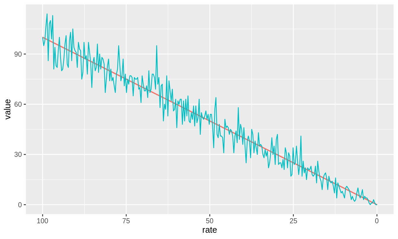
A decrease in the Poisson rate (e.g. for emission of photons) leads to a decrease in the mean (blue line) but also a decrease in fluctuations around the mean. Notice that towards the right where rate is low, fluctuations around the mean are at their smallest.

Figure 3.5: A decrease in the Poisson rate (e.g. for emission of photons) leads to a decrease in the mean (blue line) but also a decrease in fluctuations around the mean. Notice that towards the right where rate is low, fluctuations around the mean are at their smallest.

3.3 Exponential fitting detrending

Naively, one could assume that bleaching of fluorophores takes place at some constant rate. This would mean that the intensity of the image would die-off according to an exponential decay. In figure 3.6, we fit an exponential decay to such ideal data.

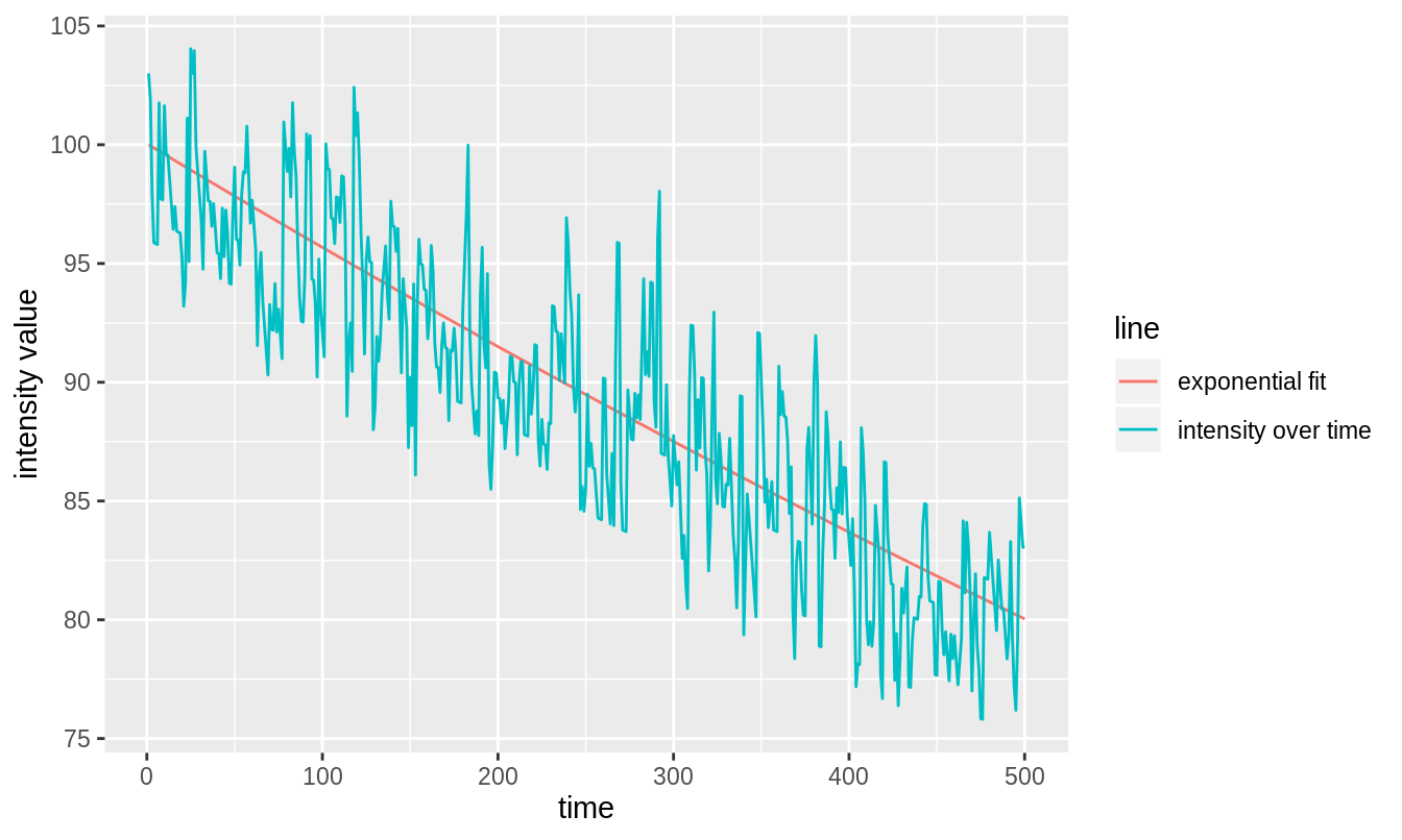
Figure 3.6: Exponential fit to intensity trace of image which is subject to bleaching at a constant rate.

Having fit the data, one may record the deviations from the fitted line as the fluctuations and replace these fluctuations about a straight line, which is placed at the mean of the original series; for figure 3.6 above, this mean is 90. Figure 3.7 shows the corrected series.

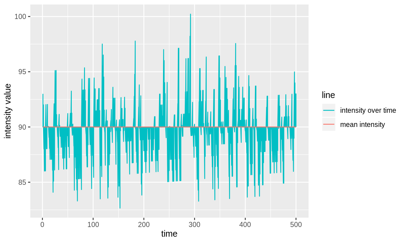
$The blue line from figure 3.6 has changed to a straight horizontal line cutting the $y$ axis at the mean intensity of the original intensity trace. The fluctuations about the blue line that existed in figure 3.6 are preserved here. As an example, see the large downward fluctuation at $t \approx 50$ seconds in both figures.$

Figure 3.7: The blue line from figure 3.6 has changed to a straight horizontal line cutting the $y$ axis at the mean intensity of the original intensity trace. The fluctuations about the blue line that existed in figure 3.6 are preserved here. As an example, see the large downward fluctuation at $t \approx 50$ seconds in both figures.

We can see that here, in the ideal case where the naive assumptions of the exponential decay fitting approach hold, this approach works quite well. Let us now examine the case where these assumptions don’t hold because there are other long-term fluctuations e.g. due to cell movement. We add these other fluctuations as a gentle sinusoid. See figure 3.8.

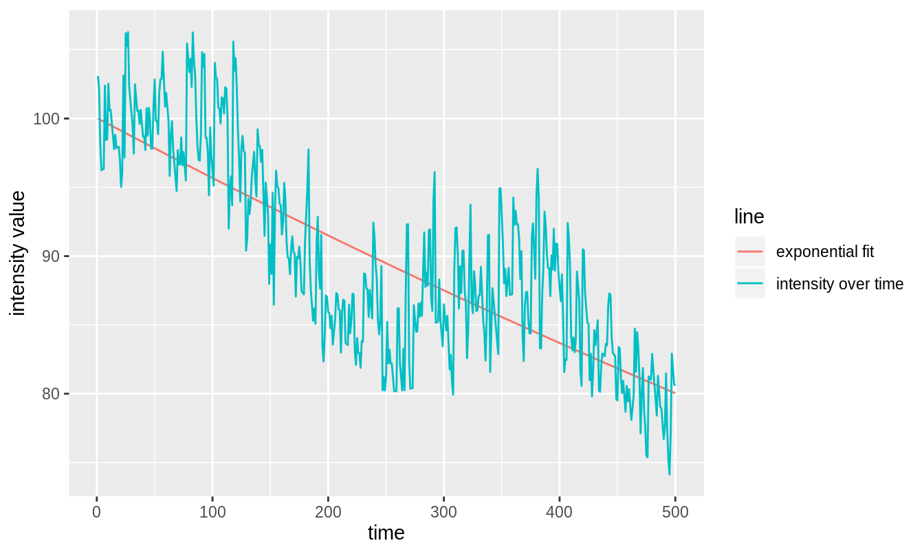
Figure 3.8: An exponential decay with added sinusoidal variance, fit with a simple exponential decay.

One can see by eye that this is not a good fit for the data. This has disastrous consequences for the detrended series, shown in figure 3.9.

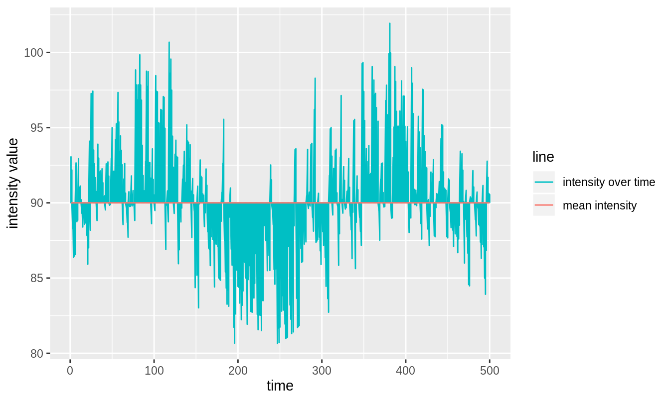
Figure 3.9: Result of exponential fitting detrending applied to a decay with a long-term sinusoidal trend component.

One can see in figure 3.9 that the exponential fit detrend failed to remove the sinusoidal trend in the data (even though it did remove the exponential decay component). We have now seen that exponential fitting detrending is appropriate when the decay has a particular form, but is otherwise not fit for use. This is a problem common to all fitting approaches to detrending, even the more flexible types like polynomial detrending (Chan, Hayya, and Ord 1977). For this reason alone, for the purpose of detrending, fitting approaches should be avoided.

3.4 Boxcar smoothing detrending

A common approach to obtaining the line from which to measure deviations/fluctuations (as in the red line in figure 3.6) is to smooth the time series, i.e. construct the line by taking a local average at each point. This is often referred to as boxcar smoothing because it can be visualized as drawing a box around a neighborhood of points, taking their average as the smoothed value at that point and then moving the box onto the next series of points and repeating the procedure; see figure 3.10.

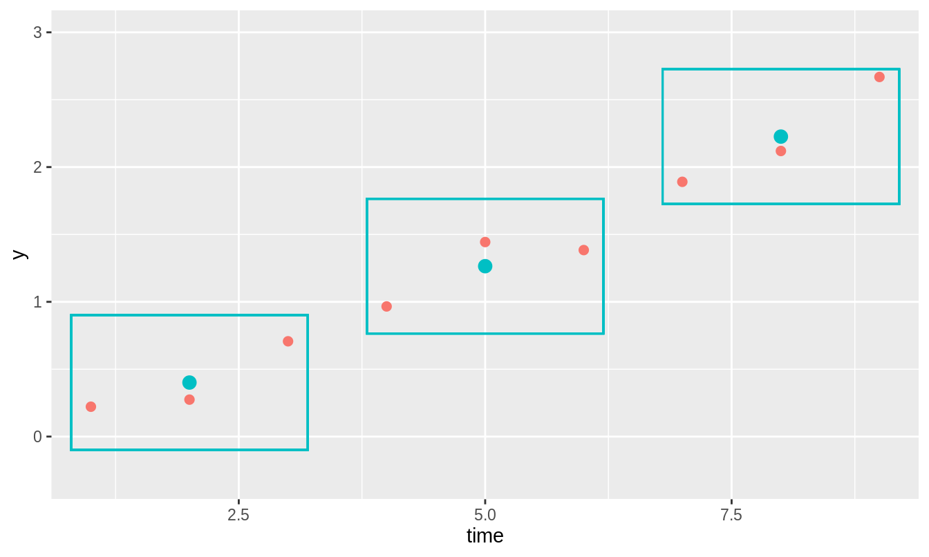
The original time series is depicted by the red dots. The blue rectangles represent the boxcar. This boxcar is said to be of length 3 because it is wide enough to encompass 3 points at a time. The boxcar is centered on a point and then the smoothed value at that point (blue dot) is calculated as the mean value of all points within the boxcar. In reality, every point gets a smoothed value which means that the boxcar overlaps but in this figure—for the sake of clarity—they are not overlapped.

Figure 3.10: The original time series is depicted by the red dots. The blue rectangles represent the boxcar. This boxcar is said to be of length 3 because it is wide enough to encompass 3 points at a time. The boxcar is centered on a point and then the smoothed value at that point (blue dot) is calculated as the mean value of all points within the boxcar. In reality, every point gets a smoothed value which means that the boxcar overlaps but in this figure—for the sake of clarity—they are not overlapped.

The length of the boxcar is equal to $2l + 1$ for natural numbered parameter $l \in \mathbb{N}$. This ensures that the length of the boxcar is always odd) which means it can always be centered upon a point). Hence the allowable lengths of a boxcar are $3,5,7,9,$ etc.

The boxcar parameter $l$ has a large effect on the type of smoothing achieved. This can be seen in figure 3.11 where boxcar smoothing is applied to the trace in figure 3.6. The traces for $l=1$ and $l=3$ are far too wiggly (not smooth enough); the trace for $l=75$ is better but perhaps still slightly wiggly; finally, the traces for $l=300$ and $l=1000$ are too close to straight horizontal lines (too smooth).

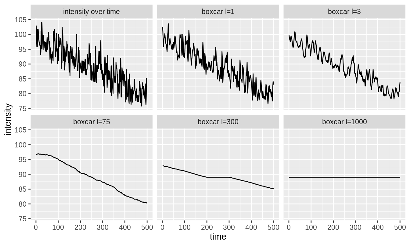
$The original intensity trace is shown in the top-left. The other panels show the result of boxcar smoothing for $l = 1, 3, 75, 300$ and $1000$. $l=1$ and $l=3$ are not smooth enough, $l = 75$ looks like it might be OK although it is slightly wiggly. $l = 300$ and $l = 1000$ are over-smoothed.$

Figure 3.11: The original intensity trace is shown in the top-left. The other panels show the result of boxcar smoothing for $l = 1, 3, 75, 300$ and $1000$. $l=1$ and $l=3$ are not smooth enough, $l = 75$ looks like it might be OK although it is slightly wiggly. $l = 300$ and $l = 1000$ are over-smoothed.

This begs the question: what is the correct smoothing parameter $l$?

3.5 The correct smoothing parameter for detrending

Figure 3.11 shows that the choice of boxcar size is crucial because different sizes lead to very different smoothed lines. The most common choice in the community is to choose $l = 10$ (Laboratory for Fluorescence Dynamics 2018). There is no justification for this choice.

In section 1.5.1, we learned that for immobile particles, the expected brightness is $B = 1$. This fact can be used to solve for the appropriate choice of $l$ to use for detrending a specific image series.

Definition 3.4 The mean intensity profile of one channel of an image series is obtained by calculating the mean intensity of each frame in that image series.

The mean intensity profile can be used to visualize the bleaching of an image series. If the fluorophores are bleaching, the mean intensity should be decreasing over time. To proceed with solving for the appropriate $l$, we need to make one assumption; this is that any two image series with the same mean intensity profile are appropriately detrended with the same detrending parameter $l$. This assumption seems reasonable, however there is no need to debate its validity because later, detrending with the solved-for parameter $l$ will be evaluated with simulated data and compared to the standard $l = 10$. If this assumption is bad, then the performance of the detrending that relies on it should also be bad. With this assumption in hand, solving for $l$ proceeds as follows:

Simulate an image series with immobile particles only which has the same mean intensity profile as the acquired real data.
Given that the simulated series is of immobile particles only, once properly detrended, it should have $B = 1$.
The $l$ for which the detrended series has mean brightness closest to 1 is the most appropriate for the simulated data.
By the assumption above, this $l$ is the most appropriate for the real data.

Mathematically, this can be expressed as

\[\begin{equation} l = \text{argmin}_{\tilde{l}} |1 - (\text{mean brightness of simulated series detrended with parameter } \tilde{l})| \tag{3.2} \end{equation}\]

In fact, what I have done here is to give a general method for solving for any detrending parameter $\alpha$:

\[\begin{equation} \alpha = \text{argmin}_{\tilde{\alpha}} |1 - (\text{mean brightness of simulated series detrended with parameter } \tilde{\alpha})| \tag{3.3} \end{equation}\]

This will be useful later when other detrending regimes with their own parameters are introduced.

3.6 Exponential smoothing detrending

Exponential smoothing is a slight alteration to boxcar smoothing. The idea is that when computing a local average, points nearer to the point of interest should have greater weights. The weights fall off with distance $|t|$ from the point of interest according to $\exp(-\frac{|t|}{\tau})$ where the parameter $\tau$ is a positive real number. This function is visualized in figure 3.12. For small values of $\tau$, only values very close to the point of interest have importance when calculating the local average. For larger values of $\tau$, further values also have importance (but closer values always have higher weights). In this sense, increasing the value of $\tau$ has a similar effect to increasing the value of $l$ for the boxcar in that further away points are taken into account.

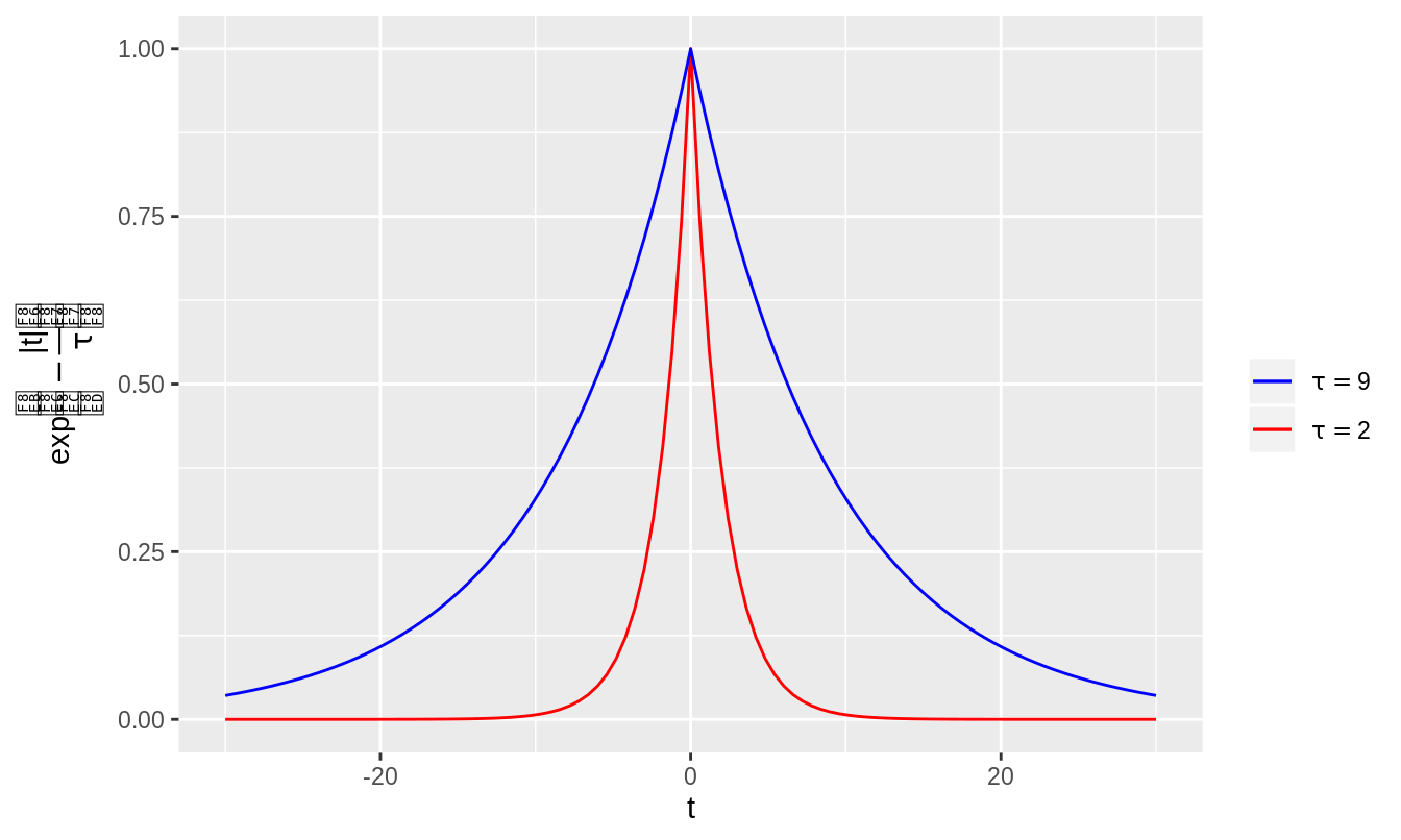
$The function $\exp(-\frac{|t|}{\tau})$ visualized with $\tau = 2$ and $\tau = 9$. For $\tau = 2$, points at distance $|t| = 10$ have approximately zero weight, whereas for $\tau = 9$, these points have significant weight.$

Figure 3.12: The function $\exp(-\frac{|t|}{\tau})$ visualized with $\tau = 2$ and $\tau = 9$. For $\tau = 2$, points at distance $|t| = 10$ have approximately zero weight, whereas for $\tau = 9$, these points have significant weight.

In figure 3.13, exponential smoothing with different parameters $\tau$ is applied to the trace in figure 3.6. The results are similar to those in figure 3.11.

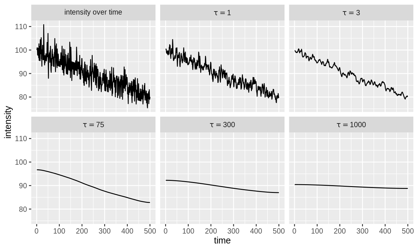
$The original intensity trace is shown in the top-left. The other panels show the result of exponential smoothing for $\tau = 1, 3, 75, 300$ and $1000$.$

Figure 3.13: The original intensity trace is shown in the top-left. The other panels show the result of exponential smoothing for $\tau = 1, 3, 75, 300$ and $1000$.

Heuristically, exponential smoothing detrending seems favorable to boxcar detrending because the idea that points further away from the point of interest are less important (but still somewhat important) when computing the local average is reasonable. Indeed, this was the method proposed in the original number and brightness paper (Digman et al. 2008). For this reason, exponential smoothing was the method of choice for my paper where the method of choosing the correct detrending parameter was published (Nolan, Alvarez, et al. 2017).

3.7 Correcting for non-stationary variance

Definition 3.5 The variance of a random variable $X$ is the expected value of the squared deviation of $X$ from its mean $\mu$: \[\begin{equation} \text{Var}(X) = E[(X - \mu)^2] \tag{3.4} \end{equation}\]

All of this chapter so far has focused on correcting for non-stationary mean. As shown in figure 3.5, as the mean decreases, so too does the variance. For an instance $x$ of the random variable $X$ with expected value $E[X] = \mu$, $x - \mu$ is the deviation of $x$ from $\mu$. If we write $x$ as $x = \mu + \tilde{x}$, then we get the deviation $x - \mu = (\mu + \tilde{x}) - \mu = \tilde{x}$, so $\tilde{x}$ is the deviation. For a given point in figure 3.5, its deviation is its distance from the red line. For positive real number $k$, making the transformation $\tilde{x} \rightarrow \sqrt{k}\tilde{x}$ i.e. $x \rightarrow \mu + \sqrt{k}\tilde{x}$ causes the variance (i.e. the squared deviation) to be transformed as $\text{Var}(X) \rightarrow k \times \text{Var}(X)$. Hence, we have a way to modify the variance of a time series as a whole by modifying the deviation of each time point from the mean. For months, I toyed with this idea as a solution of correcting for non-stationary variance. However, in reality the contribution to the variance in intensity at a given pixel is down to both Poisson photon statistics and fluorophore movement. This combination of factors makes it very difficult to ascertain the amount by which the variance should be altered. I eventually abandoned my efforts to alter the variance like this in favor of the Robin Hood detrending algorithm (section 3.9) which includes correction for non-stationary variance as an intrinsic part of its detrending routine.

3.8 Caveats of fitting and smoothing approaches

Both fitting and smoothing approaches to detrending have serious caveats. Fitting approaches assume that the fluorescence intensity decay has a certain form. Unpredictable issues such as cell movement mean that no particular decay form can be assumed. Smoothing methods do not perform well at the edges of time series that they are applied to. They also require the user to choose a smoothing parameter. The problem of how to best choose this parameter was solved recently (Nolan, Alvarez, et al. 2017), but this method has not been widely adopted. Most importantly, both fitting and smoothing fail when the data cannot be approximated as mathematically continuous (fitted and smoothed lines are continuous approximations of data). Fluorescence intensity data at low intensities—where most pixel values are either 0 or 1—are quasi-binary⁸ and hence a continuous approximation does not make sense (see figure 3.14). This means that neither fitting nor smoothing are applicable detrending methods at low intensities. This is the crucial caveat of these methods because, when bleaching is a problem, it is common to reduce laser power to reduce bleaching, which leads directly to lower intensity images. With fitting and smoothing techniques, it may sometimes be advisable to increase the laser power to achieve higher intensities such that the detrending routines will function properly. This means one may need to bleach more in order to be able to correct for bleaching. This farcical situation necessitates a new detrending technique which can function at low intensities.

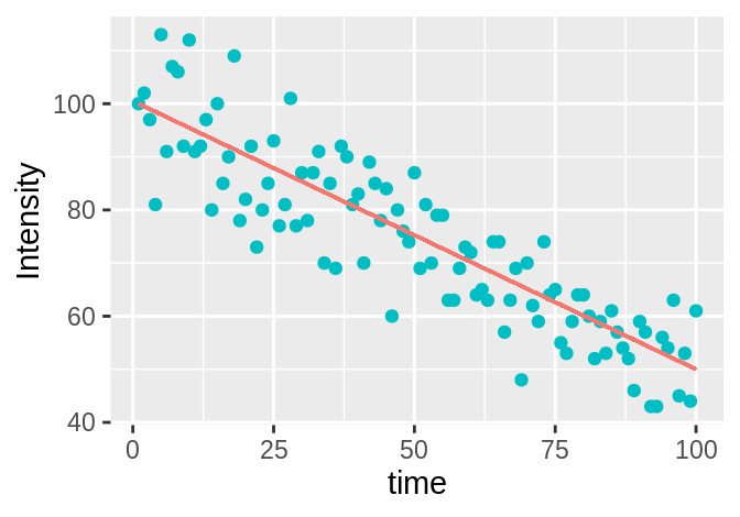
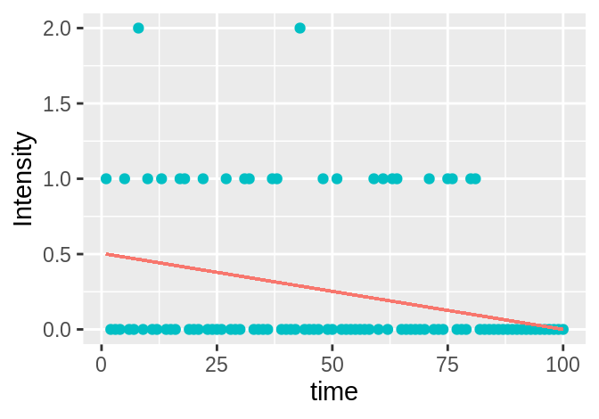
$Left: for high ($\gg 1$) intensity values, the line is a satisfactory approximation of the data, representing it well. Right: for low (quasi-binary) intensity values, the line is not a good approximation for the data and indeed no line or curve could represent the data well.$ $Left: for high ($\gg 1$) intensity values, the line is a satisfactory approximation of the data, representing it well. Right: for low (quasi-binary) intensity values, the line is not a good approximation for the data and indeed no line or curve could represent the data well.$

Figure 3.14: Left: for high ($\gg 1$) intensity values, the line is a satisfactory approximation of the data, representing it well. Right: for low (quasi-binary) intensity values, the line is not a good approximation for the data and indeed no line or curve could represent the data well.

3.9 Robin Hood detrending

Intensity images in units of photons are count data. This means that the values are all natural numbers, i.e. elements of $\mathbb{N}_0=\{0, 1, 2, 3, \ldots\}$. Fitting and smoothing give real-numbered values (elements of $\mathbb{R}$), which must then be transformed back into count data (elements of $\mathbb{N}_0$), normally by rounding. This means that fitting and smoothing methods of detrending push values through $\mathbb{N}_0 \rightarrow \mathbb{R} \rightarrow \mathbb{N}_0$ (the move back $\rightarrow \mathbb{N}_0$ is necessary because calculations like Qian and Elson’s moment analysis assume photon count data, which is necessarily in $\mathbb{N}_0$). When current methods were failing to properly detrend low-intensity images, I began to wonder was it necessary to go through the real numbers $\mathbb{R}$, given that the start and end points were the natural numbers $\mathbb{N}_0$?

Consider figure 3.15. There is a bleached and unbleached version of an intensity trace. Suppose that our real data is the bleached trace, but we wish it looked like the unbleached trace. You may wonder why the unbleached trace is not at the starting intensity of the bleached series. For reasons that will become clear, the Robin Hood algorithm can only place the detrended image at the mean intensity of the original image. This is not a problem because the issue with bleaching in FCS and FFS is mainly that the changing signal leads to incorrect calculations, not that the loss in signal leads to a critical lack of information (photons). Indeed, a feature of the Robin Hood algorithm is that it preserves the mean intensity of the real data on a pixel-by pixel basis.

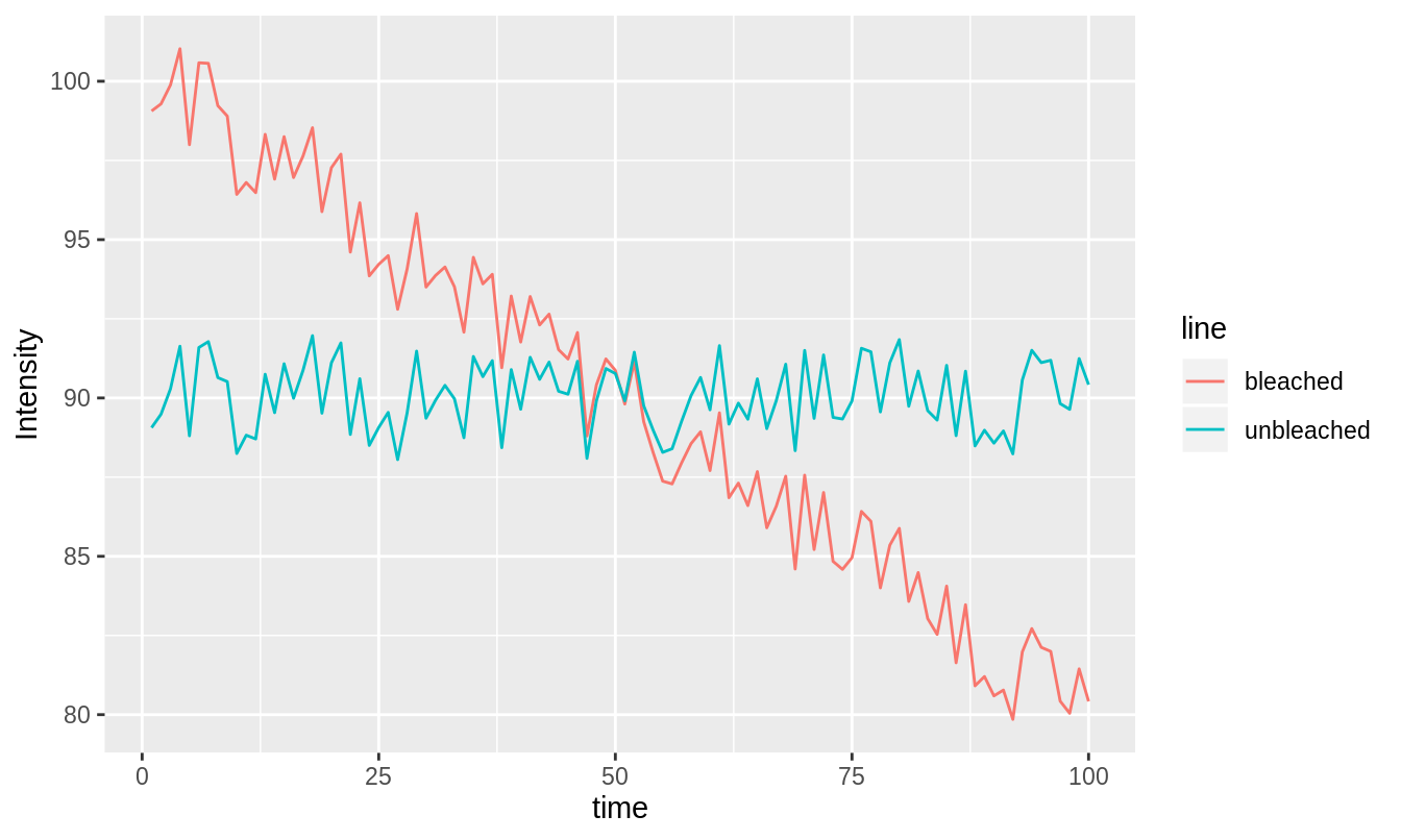
Figure 3.15: Bleached and unbleached intensity traces.

To get to the unbleached intensity trace from the bleached intensity trace, intensity must be subtracted from time-points with too much intensity and added to time points with too little intensity. This can be done by taking counts from frames with too much intensity and giving them to frames with too little intensity. In this way, no counts are gained or lost, they are just moved around the image series. See figure 3.16. Counts are passed from one frame to another along a given pixel, i.e. if a count is taken from pixel at position $p$ in some frame $i$, it must be given to a pixel at the same position $p$ in some other frame $j$. It is this condition that ensures that the mean intensity images of the original and detrended image series are the same.

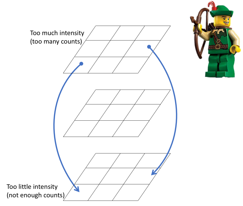
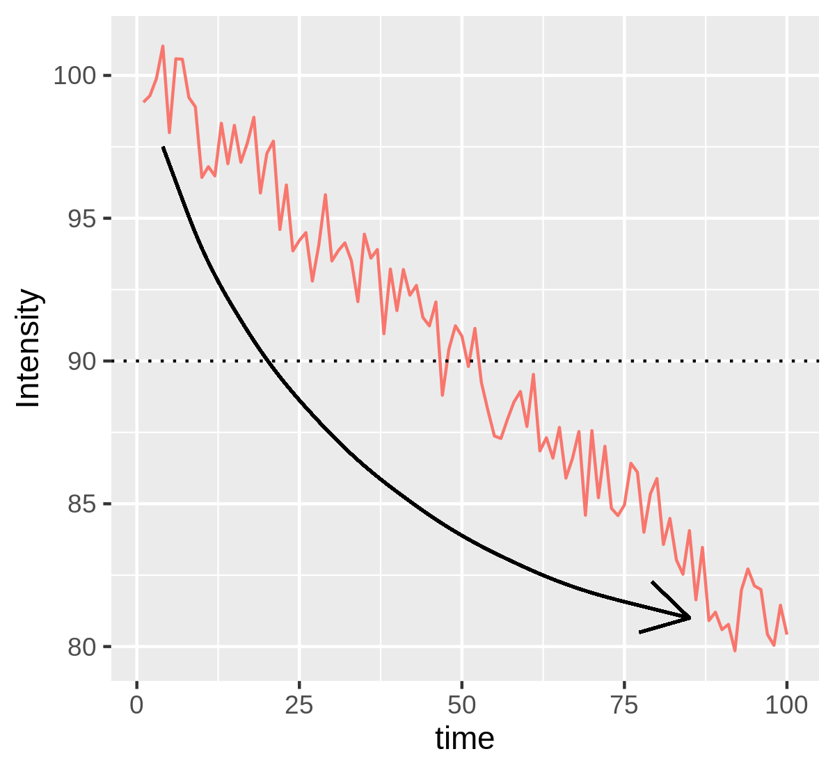
Robin Hood: counts are taken from frames of higher intensity (usually closer to the start of the image series) and given to frames of lower intensity (usually closer to the end of the image series).

Figure 3.16: Robin Hood: counts are taken from frames of higher intensity (usually closer to the start of the image series) and given to frames of lower intensity (usually closer to the end of the image series).

To determine how many swaps need to be made to detrend a given image series, equation (3.3) can be used, with $\alpha$ being the number of swaps.

The random gifting of counts from higher to lower intensity frames has the effect of temporally redistributing mean intensity but also variance in intensity. With photon statistics (which follow a Poisson distribution), random counts provide both mean and variance. This is in contrast to all previous methods which consist of determining local deviation and adding it to a fixed global mean: this provides no temporal redistribution of variance.

3.10 A comparison of detrending methods

To compare the various detrending methods, I use the following workflow:

Simulate a number $N = 100,000$ of particles diffusing with known diffusion rate. Simulations were done with the brownded software package (section 2.3.7).
Simulate photon emission from these particles with chosen brightness $\epsilon$ and create an image series from this, being careful to (virtually) sample at a rate appropriate for number and brightness analysis.
Bleach the simulation with a chosen constant bleaching rate.⁹
Simulate photon emission from the bleached simulation (bleached particles don’t emit photons) with the same brightness $\epsilon$ and create an image series.
Detrend the bleached image series.
Evaluate the detrending algorithm by measuring how close the brightness of the detrended bleached image series is to the known simulated brightness.

For all combinations of brightnesses of $\epsilon = 0.001, 0.01, 0.1, 1, 10$ and bleaching fractions of 0%, 1%, 5%, 10%, 15%, 20%, 25%, 30%, 20 images of 64x64 pixels and 5,000 frames were simulated using 100,000 fluorescent diffusing particles.¹⁰ These were detrended with the following detrending routines:¹¹

Boxcar with $l = 10$ (boxcar10, the most common detrending routine).
Exponential smoothing with automatically chosen parameter $\tau$ (autotau).
Robin Hood with automatically chosen swaps (robinhood).

The performance was evaluated using the mean relative error.

Definition 3.6 For a given brightness and bleaching fraction,

\[\begin{equation} \text{mean relative error } = \frac{|(\text{calculated brightness after detrending}) - (\text{true brightness})|}{(\text{true brightness})} \tag{3.5} \end{equation}\]

Figure 3.17 shows the results. Before I discuss them, note that the common brightnesses that we see are in the range $\epsilon = 0.003$ to $\epsilon = 0.1$.

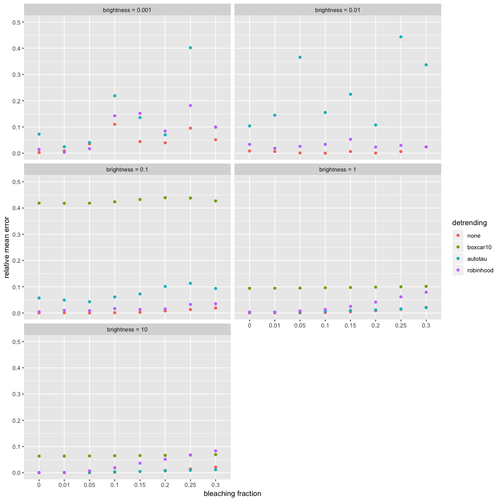
$A comparison of different detrending methods with various brightnesses and bleaching fractions (steady, constant-rate bleaching), including the results of not detrending at all.$

Figure 3.17: A comparison of different detrending methods with various brightnesses and bleaching fractions (steady, constant-rate bleaching), including the results of not detrending at all.

The most striking thing about figure 3.17 is that the best choice in all cases is to not detrend at all! This is an interesting result and seems to render all detrending routines worthless. However, when working with real data, not detrending does not work well at all. This will be shown in chapter 4. This indicated that my simulations are unrealistic. This is probably because with real data, bleaching is likely not taking place at a constant, steady rate and other factors such as cell movement or/and laser power fluctuations are contributing to medium and long term intensity fluctuations and these have a detrimental effect on calculations if not detrended out. It would be possible to study this by mimicking real bleaching profiles with simulations (see section 6.2).

The worst performer by far is boxcar10. For example, at $\epsilon = 0.1$, it makes an error of worse than 40% and for $\epsilon = 0.001, 0.01$, its error is worse than 50%, so it does not even appear on the plot. This is good evidence that arbitrarily choosing the parameter $l$ is very bad practice. For realistic brightnesses ($\le 0.1$), robinhood is the best with errors almost always lower than 5%. autotau also performs very well, with errors almost always less than 10%. At the lowest brightness $\epsilon = 0.001$, all methods are somewhat erratic. That is because at this extremely low brightness, there is a critical lack of information (photons) for the algorithms to work with. Finally, at unrealistically high brightnesses of $\epsilon = 1, 10$, autotau begins to perform well because at these high photon counts, the caveats of smoothing have totally disappeared. However, I cannot explain the degradation in the performance of robinhood in this case. Fortunately, there is no need to dwell on this, as this situation ($\epsilon = 1, 10$) does not arise in practice because available fluorophores are not this bright.

References

Chan, K. Hung, Jack C. Hayya, and J. Keith Ord. 1977. “A Note on Trend Removal Methods: The Case of Polynomial Regression Versus Variate Differencing.” Econometrica 45 (3). JSTOR: 737. doi:10.2307/1911686.

Digman, M. A., R. Dalal, A. F. Horwitz, and E. Gratton. 2008. “Mapping the number of molecules and brightness in the laser scanning microscope.” Biophys. J. 94 (6): 2320–32. doi:10.1529/biophysj.107.114645.

Laboratory for Fluorescence Dynamics. 2018. Globals for Images: SimFCS 4. University of California, Irvine. http://www.lfd.uci.edu/globals/.

Nolan, Rory, L Alvarez, Jonathan Elegheert, Maro Iliopoulou, G Maria Jakobsdottir, Marina Rodriguez-Muñoz, A Radu Aricescu, and Sergi Padilla Parra. 2017. “Nandb—number and Brightness in R with a Novel Automatic Detrending Algorithm.” Bioinformatics 33 (21). Oxford University Press: 3508–10. doi:10.1093/bioinformatics/btx434.

By quasi-binary, I just mean that almost all values are 0 or 1.↩
It would be good to test with non-constant bleaching rates too, this wasn’t done due to time constraints.↩
The simulation took 3 weeks.↩
The detrending took 2 weeks.↩